Hi, and welcome!
We love pixels. We build our tools such that they allow us to work with pixels at a wide range of scales, from individual landsat scenes, to global mosaics, via command line programs or as python libraries we can integrate into large processing pipelines.
Today we'll walk through:
- processing an individual Landsat scene using rasterio, a tool which serves as the foundation for most of our work
- uploading the outputs of ^ to Mapbox, where we can visualize it on top of
mapbox.satellite, and serve it globally at crazy speed
There are all sorts of ways to get Landsat 8 data. The best solution is going to depend on what you're trying to accomplish. For working with individual scenes like we'll do today, we're going to visually search for data. For larger pipelines, like Landsat Live, you'll want a more programmatic approach; we'll talk briefly about options for doing so.
So. Many. Options!
To start, let's use EarthExplorer.
- Search for Santa Barbara, filter on Landsat 8 data, and note the Path and Row of a Landsat scene that intersects it.
But rather than using EarthExplorer to download the data, let's use Landsat on AWS.
- In order to download data from EE, you'll need to create an account
- You'll need to download all of the data for the scenes you're interested in, rather than just the bands you're particularly interested in.
Let's get some data.
- Open your terminal
- Make two new directories for your data with
mkdir 042-035 && mkdir 042-036 - Head over to Landsatonaws.com, download the 7, 5, 4, 3, and 2 bands, and move the data into the appropriate directory.
- Shortcut: the path is going to look like
landsatonaws.com/L8/042/036
- Shortcut: the path is going to look like
The greater the volume of data you're going to work with, the more time you'll save by automating this workflow. We won't go into too much detail, but if you're interested, check out:
- The
awsclimethod as described here. - landsat-util
- sat-utils/sat-api
- RemotePixel/aws-sat-api
Each Landsat 8 scene will have a total of 12 tif files. Each tif maps to a particular band, which more or less represents a unique segment of the electromagnetic spectrum. We can mix and match different combinations of bands to generate composites which can help us to understand reality in different ways.
Today, we're going to build 2 composites
432— Natural color- 4: Red
- 3: Blue
- 2: Green
752— Fire scars- 7: Red
- 5: Blue
- 2: Green
Broadly, a TIF consists of metadata and data.
- Let's use Rasterio to inspect the metadata for one of these bands.
$ rio info --indent 2 LC08_L1TP_042036_20171209_20171209_01_RT_B2.TIF
{
  "driver": "GTiff",
  "dtype": "uint16",
  "nodata": null,
  "width": 7831,
  "height": 7961,
  "count": 1,
  "crs": "EPSG:32611",
  "transform": [
    30.0,
    0.0,
    121185.0,
    0.0,
    -30.0,
    3952515.0
  ],
  "blockxsize": 512,
  "blockysize": 512,
  "tiled": true,
  "compress": "deflate",
  "interleave": "band",
  "shape": [
    7961,
    7831
  ],
  "bounds": [
    121185.0,
    3713685.0,
    356115.0,
    3952515.0
  ],
  "res": [
    30.0,
    30.0
  ],
  "lnglat": [
    -119.85005844764973,
    34.60649717059448
  ]
}
"dtype": "uint16" refers to the range of pixels that could represent pixel values in any of the tifs.
2 ^ 16 == 65,536 # because computers, we're going to represent this range as 0 to 65,535This is a problem! It's tough to represent 16bit images on the web. Our hooman eyes don't really distinguish much beyond 255 values per color channel, so the common image formats used on the internet don't either.
We're going to need to convert the pixels in our data from 16bit to to 8bit, which in computer, works out to a total of 255 values.
- Use
rio convertto scale the data from 16bit to 8bit.
$ rio convert LC08_L1TP_042036_20171209_20171209_01_RT_B2.TIF 2.tif \
    --dtype uint8 \
    --scale-ratio 0.0039  # 255 / 65536 == 0.0039
Let's check the metadata again!
$ rio info --indent 2 2.tif | jq .dtype
"uint8"
Now that we have less data, these files are quite a bit smaller too!
$ ls -lh
-rw-r--r--  1 jacques  staff   7.0M Dec 12 13:08 2.tif
-rw-r--r--@ 1 jacques staff 52M Dec 11 12:42 LC08_L1TP_042036_20171209_20171209_01_RT_B2.TIF- Repeat this process for the remaining bands.
These bands will be a whole lot more interesting to look at once we've stacked them together into a single RGB image.
$ rio stack 4.tif 3.tif 2.tif 432.tif --rgb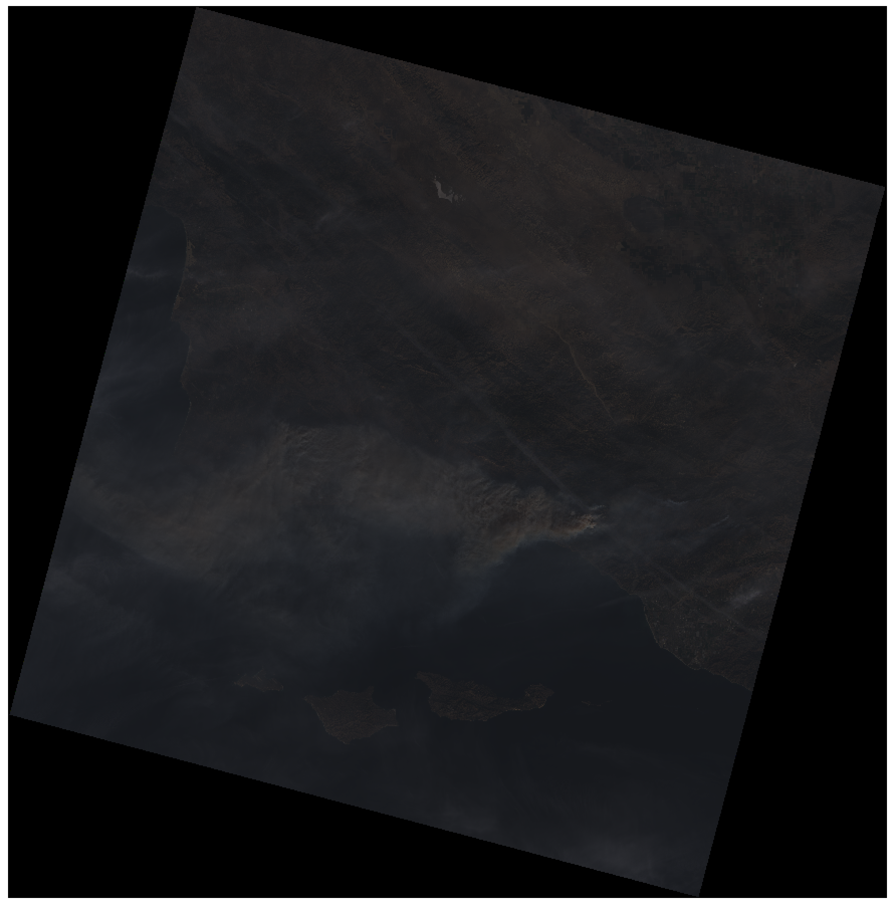
Creation options
The --rgb flag here is an alias for a --co PHOTOMETRIC=rgb flag. Rasterio supports the full range of GDAL creation options. Most of these options affect the internal structure of the tif itself. We'll use more of these later!
For this Landsat scene, the data we actually care about sits in an island of black data, where the Landsat sensors didn't actually collect any data. These pixels are represented as pure black pixels, which have RGB values of [0, 0, 0].
$ rio info --indent 2 432.tif | jq .nodata
null
If we display this imagery as is on top of mapbox.satellite, those black pixels are going to be included. We don't want that. To "hide" them, we can update the raster's metadata to indicate that regions with RGB stacks that equal [0, 0, 0] should be excluded.
$ rio edit-info --nodata 0 432.tifIf we inspect the data again, we'll see that our metadata has changed.
$ rio info --indent 2 432.tif | jq .nodata
0One of the wonderful things about Rasterio is that it's very easy to build plugins on top of it. For instance, we can use rio-color to tweak the color of these images.
- Install
rio-colorwithpip install rio-color - Use the new
rio atmoscommand to apply a few standard corrections to your composite.
$ rio atmos 432.tif 432-dehazed.tif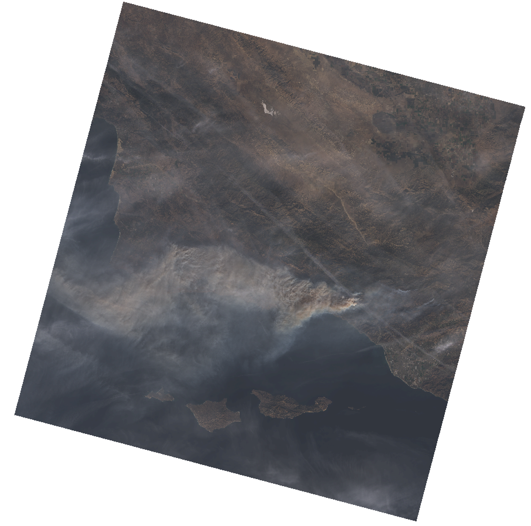
- Let's upload this image to Mapbox. You'll need to sign up for account if you don't already have one.
You could create a new tileset directly in the browser, but for now let's stsay on the command line a bit longer.
- Install the
mapbox-cli
You'll need to provide an Access Token in order to interact with your Mapbox account.
From here, we can upload our data directly.
$ mapbox upload jacques.santa-barbara-432 432-dehazed.tifOur 432 composite shows the smoke well, but it's difficult to pinpoint the fire itself. Let's build a 752 composite, which should let us "see" it a bit more clearly.
$ rio stack 7.tif 5.tif 2.tif 752.tif --rgbWe're going to have the same nodata issue...
$ rio info --indent 2 7.tif | jq .nodata
null
...but let's address it a little differently this time.
- Install rio-alpha with
pip install rio-alpha
Rather that amending the metadata, such that all [0, 0, 0] pixels are identified as nodata, we're going to create an alpha band.
$ rio alpha 752.tif --ndv 0 752A.tifLet's check out the metadata again.
rio info --indent 2 752A.tif | jq ".colorinterp"
[
  "red",
  "green",
  "blue",
  "alpha"
]
We've added an entirely new band! This new band acts as a mask over all the regions we would have previously identified as nodata.
Like we did before, let's use rio atmos to enhance the color a bit.
$ rio atmos 752A.tif 752A-dehazed.tifSo far, we've worked on the scale of a single Landsat scene. This doesn't always provide us with full scope of the context we need.
Let's switch from our 042-036 scene to 042-035 scene and process a 752 composite for it as well.
- Ask questions if you get stuck!
Once you're finished, let's go ahead and merge the data together.
$ rio merge 042-035/752A-dehazed.tif 042-036/752A-dehazed.tif out.tif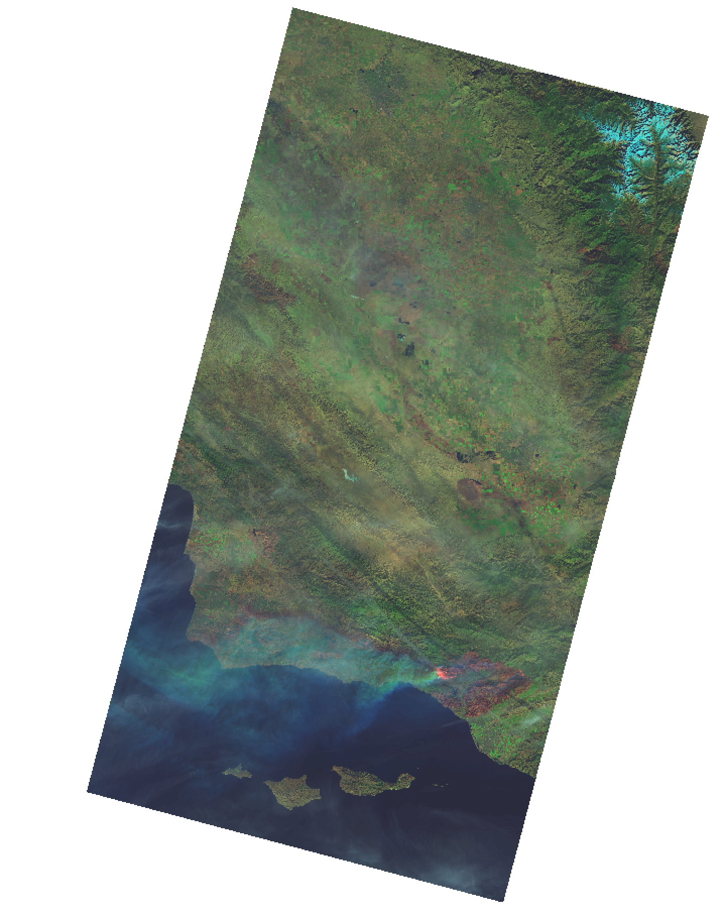
All sorts of directions you could go:
- Create a composite using imagery from before the Fire, and compare tilesets from before and after.
- Check out landsat-tiler, which let's you:
- Process the Landsat 8 imagery on AWS rather than your laptop
- Automatically cuts and serves tiles for you 🙂
- Take a look at Planet's imagery of the fires
Thanks!