covidfrance_shiny.R

library(leaflet)
library(sf)
library(rmapshaper)
library(dplyr, warn.conflicts = FALSE)
library(smoothr)
library(shiny)

u <- httr::GET('https://www.data.gouv.fr/api/1/datasets/5e7e104ace2080d9162b61d8/')
url_search <- httr::content(u)$resources

df_date <- tibble(url = url_search %>% purrr::map_chr('url'),
                  timestamp = url_search %>% purrr::map_chr('last_modified')) %>% 
    filter(grepl('hospitalieres-covid', url)) %>% 
    arrange(desc(timestamp)) %>% 
    pull(timestamp) %>% 
    .[1] %>% 
    lubridate::as_datetime() %>% 
    format(., '%Y-%m-%d à %Hh%Mm')

dat_cov <- readr::read_csv2('https://www.data.gouv.fr/fr/datasets/r/63352e38-d353-4b54-bfd1-f1b3ee1cabd7') %>% 
    filter(sexe == 0) %>% 
    filter(!is.na(jour)) %>% 
    select(dep, jour, hosp, rad, rea, dc)

ui <- bootstrapPage(
    
    tags$head(
        tags$link(href = "https://fonts.googleapis.com/css?family=Oswald", rel = "stylesheet"),
        tags$style(type = "text/css", "html, body {width:100%;height:100%; font-family: Oswald, sans-serif;}"),
        #includeHTML("meta.html"),
        tags$script(src="https://cdnjs.cloudflare.com/ajax/libs/iframe-resizer/3.5.16/iframeResizer.contentWindow.min.js",
                    type="text/javascript")),
    
    leafletOutput("covid", width = "100%", height = "100%"),
    
    absolutePanel(
        bottom = 20, left = 40, draggable = TRUE, width = "20%", style = "z-index:500; min-width: 300px;",
        titlePanel("France | Covid"),
        # br(),
        em('La donnée est affichée en plaçant la souris sur la carte'),
        sliderInput("jour",h3(""),
                    min = min(dat_cov$jour), max = max(dat_cov$jour), step = 1, 
                    value = max(dat_cov$jour),
                    animate = animationOptions(interval = 1700, loop = FALSE)),
        tags$style(".form-control {background-color: #d4dcdc !important; color: #333}"),
        dateInput(
            inputId = "date_1", 
            # value = min(dat_cov$jour),
            value = '2020-06-01',
            weekstart = 1,
            startview = "year",
            label = "Date de début",
            format = "D dd/mm/yyyy",
            min = min(dat_cov$jour),
            language = "fr",
            max = Sys.Date()
        ),
        shinyWidgets::prettyRadioButtons('sel_data', 'Donnée affichée', 
                                         choices = c('Hospitalisés', 'En réanimation', 'Retours à domicile (cumulés depuis 1ère vague)', 'Décès (cumulés depuis 1ère vague)'), 
                                         selected = 'Hospitalisés', 
                                         shape = "round", animation = "jelly",plain = TRUE,bigger = FALSE,inline = FALSE),
        shinyWidgets::prettySwitch('pop', "Ratio / 100 000 habitants*", FALSE),
        em(tags$small("*à noter sur ce ratio : un patient peut être hospitalisé plus d'une fois")),
        em(tags$small(br(), "Pour les décès, il s'agit de ceux ayant lieu à l'hôpital")),
        h5(tags$a(href = 'http://github.com/GuillaumePressiat', 'Guillaume Pressiat')),
        
        h5(em('Dernière mise à jour le ' , df_date)),
        
        #br(),
        tags$small(tags$li(tags$a(href = 'https://www.data.gouv.fr/fr/datasets/donnees-hospitalieres-relatives-a-lepidemie-de-covid-19', 'Données recueil Covid')),
                   tags$li(tags$a(href = 'https://github.com/gregoiredavid/france-geojson', 'Geojson contours départements')),
                   tags$li(tags$a(href = 'https://www.insee.fr/fr/statistiques/2012713#tableau-TCRD_004_tab1_departements', 'Populations Insee')),
                   tags$li(tags$a(href = 'http://r.iresmi.net/2020/04/01/covid-19-decease-animation-map/', 'Voir également ce lissage territorial')),
                   tags$li(tags$a(href = 'http://www.fabiocrameri.ch/resources/ScientificColourMaps_FabioCrameri.png', 'Scientific colour maps'), ' with ',
                           tags$a(href = 'https://cran.r-project.org/web/packages/scico/index.html', 'scico package'))))
    
    
)


#data.p <- sf::st_read("Downloads/contours-simplifies-des-departements-francais-2015.geojson") %>% 
# https://raw.githubusercontent.com/gregoiredavid/france-geojson/master/departements.geojson
# data.p <- sf::st_read("https://raw.githubusercontent.com/gregoiredavid/france-geojson/master/departements-avec-outre-mer.geojson") %>%
# #  filter(! code_reg %in% c('01', '02', '03', '04', '06')) %>%
#   ms_simplify(keep = 0.03) %>%
#   smooth(method = "chaikin")

pops <- readr::read_csv2('pop_insee.csv')

#st_write(data.p, 'deps.geojson', delete_dsn = TRUE)
 data.p <- st_read('deps.geojson')

data <- data.p %>% 
    #left_join(dat_cov, by = c('code_dept' = 'dep')) %>% 
    left_join(dat_cov, by = c('code' = 'dep')) %>% 
    left_join(pops, by = c('code' = 'dep'))


server <- function(input, output, session) {
    
    dataa <- reactive({
        data %>% filter(jour >= input$date_1)
    })
    
    observeEvent({input$date_1}, {
    updateSliderInput('jour', min = input$date_1, session = session)
    })
    
    get_data <- reactive({
        temp <- dataa()[which(dataa()$jour == input$jour),]
        if (input$sel_data == "Hospitalisés"){
            temp$val <- temp$hosp
        } else if (input$sel_data == "En réanimation"){
            temp$val <- temp$rea
        } else if (input$sel_data == "Retours à domicile (cumulés depuis 1ère vague)"){
            temp$val <- temp$rad
        } else if (input$sel_data == "Décès (cumulés depuis 1ère vague)"){
            temp$val <- temp$dc
        } 
        
        
        
        temp$label <- temp$val
        
        if (input$pop){
            temp$val <- (temp$val * 100000) / temp$pop2020
            temp$label <- paste0(temp$label, '<br><em>', round(temp$val,1), ' / 100 000 hab.</em><br>', prettyNum(temp$pop2020, big.mark = ' '), ' habitants')
        }
        
        temp <- temp %>% filter(jour >= input$date_1)
        return(temp)
        
    })
    values_leg <- reactive({
        temp <- dataa()
        if (input$sel_data == "Hospitalisés"){
            temp$leg <- temp$hosp
        } else if (input$sel_data == "En réanimation"){
            temp$leg <- temp$rea
        } else if (input$sel_data == "Retours à domicile (cumulés depuis 1ère vague)"){
            temp$leg <- temp$rad
        } else if (input$sel_data == "Décès (cumulés depuis 1ère vague)"){
            temp$leg <- temp$dc
        } 
        if (input$pop){
            temp$leg <- (temp$leg * 100000) / temp$pop2020
        }
        temp <- temp$leg
        # if (input$log){
        # temp <- log(temp)
        # temp[temp < 0] <- 0
        # }
        return(temp)
    })
    
    leg_title <- reactive({
        if (input$pop){
            htmltools::HTML('Nb pour<br>100 000 hab.')
        } else{
            'Nb'
        }
    })
    
    output$covid <- renderLeaflet({
        leaflet(data = data.p) %>%
            addProviderTiles("CartoDB", options = providerTileOptions(opacity = 1, minZoom = 3, maxZoom = 7), group = "Open Street Map") %>%
            setView(lng = 1, lat = 46.71111, zoom = 6) %>%
            addPolygons(group = 'base', 
                        fillColor = NA, 
                        color = 'white',
                        weight = 1.5)  %>%
            addLegend(pal = pal(), values = values_leg(), opacity = 1, title = leg_title(), 
                      position = "topright")
    })
    
    
    
    pal <- reactive({
        
        if (input$sel_data != "Retours à domicile (cumulés depuis 1ère vague)"){
            return(colorNumeric(scico::scico(n = 300, palette = "tokyo", direction = - 1, end = 0.85), values_leg(), na.color = NA))
        } else { 
            return(colorNumeric(scico::scico(n = 300, palette = "oslo", direction = - 1, begin = 0.2, end = 0.85), domain = values_leg(), na.color = NA))
        }
    })
    
    
    observe({
        if(input$jour == min(dat_cov$jour)){
            data <- get_data()
            leafletProxy('covid', data = data) %>%
                clearGroup('polygons') %>%
                addPolygons(group = 'polygons', 
                            fillColor = ~pal()(val), 
                            fillOpacity = 1, 
                            stroke = 2,
                            color = 'white',
                            weight = 1.5, label = ~ lapply(paste0("<b>", code, " - ", nom, "</b><br>",jour, ' : ', label), htmltools::HTML))
        } else {
            data <- get_data()
            leafletProxy('covid', data = data) %>%
                #clearGroup('polygons') %>%
                addPolygons(group = 'polygons',
                            fillColor = ~pal()(val), 
                            fillOpacity = 1, 
                            stroke = 2,
                            color = 'white',
                            weight = 1.5, label = ~ lapply(paste0("<b>", code, " - ", nom, "</b><br>",jour, ' : ', label), htmltools::HTML))
        }
        
    })
}

# Run the application 
shinyApp(ui = ui, server = server)

https://guillaumepressiat.shinyapps.io/covidfrance/

This is one of the coolest app I've seen recently!

Nice use of map as a full background 🤩...and the animations 🤯

👏

Thank you for your nice comment ! Appreciate that.

In case other are looking at gist, supplementary data (pops) used in app:

library(dplyr)
# to get pop_insee.csv
url <- "https://www.insee.fr/fr/statistiques/fichier/2012713/TCRD_004.xls"

tmp <- tempfile()

download.file(url, tmp, mode = "wb")

pops_raw <- readxl::read_excel(tmp, skip = 3)

pops <- pops_raw %>%
  select(dep = 1, pop2020 = 3)

unlink(tmp)

Yes, it's an alternative to have it automatically.
Thank you.

But this data won't change in 2020 so a bit risquy to download it each time the app is build in my opinion I found (some reasons: it downloads the file repetively; if site is down; if file format has changed).

Agree; just to get the app to work initially - download once and save locally 😅

Thanks for this great app Guillaume!

For your information, I have included it in my collection of top R resources on Covid-19.

Don't hesitate to let me know if there is any inconsistency or if you prefer that I don't mention it.

Thank you very much.

Ok for me, nice!

Congratulations for this app.
I'm new to R and I studied its code, but I had difficulties to reproduce it on my computer. I downloaded the files contours-simplifies-des-departements-francais-2015.geojson and TCRD_004.xls, but I still haven't managed to generate the app.
The return message:
Warning: Error in paste0: object 'nom' not found
Can you help me?

The nom variable comes from the data.p, which is sourced from this data.

Thank you @leungi.

If it's not ok for you @fsvm78, I will create a repo with all files and a preparation data script. Better way I think.

Have you correctly saved pop file in csv ?

My csv is like this:

Tell me.

Guillaume

Thanks, GuillaumePressiat and leungi!
I'll try here.

Hi GuillaumePressiat!
I'm having trouble to creating simplest map with my data. Can you help me?
Here my code:

library(shiny)
library(RColorBrewer)
library(dplyr)
library(rgdal)

My dataset, like yours, has a code for the municipality (CD_MUN), occurrence dates (DATA) and the value I want to display (Indice_positividade)

dataset <- read.csv(file = "./br_covid/dataset.csv", stringsAsFactors = FALSE) %>%
	select(Codigo_IBGE, Sigla_Estado, cidade, longitude, latitude, Data, Total_Exames, Total_positivos, Indice_Positividade)
dataset$Data <- as.Date(dataset$Data)
dataset$Codigo_IBGE <- as.character(dataset$Codigo_IBGE)

ui <- fluidPage(
    titlePanel("Meu mapa"),
    sidebarLayout(
    sidebarPanel(
       sliderInput(inputId = "Data",
                  label = "Data:",
                  min = min(dataset$Data),
                  max = max(dataset$Data),
                  value = max(dataset$Data))
    ),

    mainPanel(

      leafletOutput(outputId = "mapa", width = "100%", height = 400)

    )
  )
)

my polygons
data.p <- st_read('./br_covid/br_municipios.geojson')

join with my dataset
casos <- data.p %>% left_join(dataset, by = c('CD_MUN' = 'Codigo_IBGE'))

show only polygons that have information after joining
casos <- subset(casos, casos$longitude != "NA")

server <- function(input, output) {

  output$mapa <- renderLeaflet({

	pal_fun <- colorBin("YlOrRd", domain = 0:100, bins = c(0, 10, 20, 35, 50, 65, 85, 100), pretty = FALSE)

	p_popup1 <- paste(sep="","<b>", data$cidade,"</b>",
                         "<br/>","<font size=2 color=#045FB4>","Número de exames: ","</font>", data$Total_Exames,"</font>",
				 "<br/>","<font size=2 color=#045FB4>","Número de casos positivos: ","</font>", data$Total_positivos,"</font>")


	leaflet(casos)%>% 
	addTiles() %>% 
	addPolygons(color = "Black", weight = 1, fillColor = ~pal_fun(Indice_Positividade), fillOpacity = 0.8, smoothFactor = 0.5, popup = p_popup1) %>%  
	addLegend("bottomright", pal = pal_fun, values = ~Indice_Positividade, title = 'Positivos/total de Exames(%) por município', labFormat = labelFormat(suffix = '%', between = '% - '))

  })

}

shinyApp(ui = ui, server = server)

Thanks, Fred

Hi Fred,

Without data it's not easy to help but

I see that you're calling in leaflet an object named data that is not defined before ?

Hope this helps.

Otherwise can you share your data ?

Guillaume

Hi Guillaume Pressiat,

Thanks for help. This is my data.

Brasil geoJson (very large)
https://drive.google.com/file/d/1re9Km7JHXX6Vtxnz3UyE3l7SXZD9NSQj/view?usp=sharing

My brief dataset
https://drive.google.com/file/d/1abb7sc5pbhoPj_fwqHBkeXN3TyXVIE1p/view?usp=sharing

My script.R
https://drive.google.com/file/d/1MMVgS1wQg9hWkPHPMsRbbJfiwt6WcA_H/view?usp=sharing

Fred

Hi,

I think municipios are too many to learn correctly a map with leaflet (in a first approach). And this shapefile (geojson) is really big. All code will run too slow to iterate your process. Trying with less polygons first is a better way to print your data (I think), step by step.

I have found here a shapefile for UF (I'm not an expert, looking at this from France).

library(shiny)
library(RColorBrewer)
library(dplyr)
# library(rgdal)
library(leaflet)
library(sf)
library(rmapshaper)
# install.packages('rmapshaper')

dataset <- read.csv(file = "dataset_res.csv", stringsAsFactors = FALSE, encoding = 'latin1') %>%
	select(Codigo_IBGE, Sigla_Estado, cidade, longitude, latitude, Data, Total_Exames, Total_positivos, Indice_Positividade)
dataset$Data <- as.Date(dataset$Data)
dataset$Codigo_IBGE <- as.character(dataset$Codigo_IBGE)

# for one day first
dataset1 <- dataset %>% 
  filter(Data == as.Date('2020-03-10'))

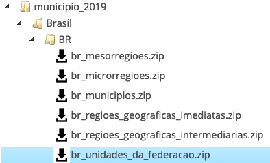
data_uf <- st_read('br_unidades_da_federacao', layer = 'BR_UF_2019')
# plot(data_uf)

# Summarise by UF
dataset1 <- dataset1 %>% 
  group_by(Sigla_Estado) %>% 
  summarise(Total_positivos = sum(Total_positivos, na.rm = TRUE))

data_uf <- data_uf %>% ms_simplify(keep = 0.1)
#plot(data_uf)

casos <- data_uf %>% left_join(dataset1, by = c('SIGLA_UF' = 'Sigla_Estado')) %>% 
  mutate(popup = paste0(SIGLA_UF," -", NM_UF, " : ", Total_positivos))

# plot(casos)

pal_fun <- colorNumeric("YlOrRd", domain = as.integer(1:max(casos$Total_positivos, na.rm = TRUE)),na.color = NA)

casos <- sf::st_transform(casos,sp::CRS('+proj=longlat +datum=WGS84'))

leaflet(casos) %>% 
  addTiles() %>% 
  addPolygons(color = 'black', weight = 1, fillColor = ~pal_fun(Total_positivos), 
              fillOpacity = 0.8, smoothFactor = 0.5, label = ~ popup) %>% 
  addLegend("bottomleft", pal = pal_fun, values = ~Total_positivos, 
            labFormat = prettyNum,
            title = 'Total Positivos de Exames por UF')

It works for me, if ok for you then maybe next step by municipios (or join by UF/municipios to jump on microrregioes, mesorregioes) ?

For "covidfrance", areas are departments, n = 100.

leafgl is maybe better for printing a leaflet with many polygons (n > 1000 for instance).

you should also take a look at rmapshaper or another package to simplify a bit your shapefile before running leaflet like it's done here data_uf <- data_uf %>% ms_simplify(keep = 0.1).

Thanks GuillaumePressiat for the help and tips, but I needed to understand how to use shiny to see my data on different days. There's something in my script that doesn't work.
https://drive.google.com/file/d/1MMVgS1wQg9hWkPHPMsRbbJfiwt6WcA_H/view?usp=sharing

For purposes, for example, you can use the federation geojson (29MB) that I provide in the link below ( converted .geojson AND wgs 84).
https://drive.google.com/file/d/1cyc8brSC_9Fd_66JT9cZP3NwiRWpLd1B/view?usp=sharing

Regarding the size and number of polygons in .geojson, the alternative was to create an object (map) that showed only the polygons that had information (except NA) after the left join function (geojson + data set). In this case, on 2020-03-10 it would be only 561 polygons and on 2020-03-11 it would be 560 polygons.

casos <- subset(casos, casos$longitude != "NA"

That was a way to make things easier for the leaflet, but I'll look at rmapshaper and leafgl.

If you can, help me find out why my shiny script doesn't work.

Thank you!

Fred

Hi, GuillaumePressiat, in your code
data <- data.p %>%
#left_join(dat_cov, by = c('code_dept' = 'dep')) %>%
left_join(dat_cov, by = c('code' = 'dep')) %>%
left_join(pops, by = c('code' = 'dep'))

the result data seems not including the geometry, I am wondering how you achieve it.
while I did similar things with df and geojson, the result merged data is always a geojson format.

can you give me a little hint? thanks!

Hi Halfbakedpanda,

I think this is because I read the geojson shapes with a recent sf package and not with rgdal as before.

But geometry is inside the tibble embedded as a list, see

It seems to work like this!

Prompt reply! Thanks, and I now tried the same on US states level covid data
(source from https://github.com/CSSEGISandData/COVID-19/tree/master/csse_covid_19_data/csse_covid_19_daily_reports_us)
and us.census data ( https://www2.census.gov/programs-surveys/popest/datasets/2010-2019/state/detail/SCPRC-EST2019-18+POP-RES.csv) with the geojson (https://raw.githubusercontent.com/jgoodall/us-maps/master/geojson/state.geo.json).

but the backend usually takes an interval of 7000 (7 seconds) to refresh when I change any of the input. I am wondering is this normal? and any suggestion for making it faster?

I guess it might because my geojson file is to complicated (many features). and the merged dataframe also become complicated.

anyway, really thanks, have learned a lot from your project.

Hi,

You have to simplify your shape file I think.

Whereas for @fsvm78 there are maybe too many shapes on his level, for US-states level it's ok. (100 departments in France, so ~50 states is ok).

For US-counties level (a better level to see more precisely COVID in this big country?), leafgl maybe is a package to consider.

But for states, it should work with your data.

Another thing to consider is to keep only variables that you will use for the data you have to put inside the shiny app server, same thing for leaflet maps.

You can run something like this to simplify and smooth (one time) your shapefile.

library(leaflet)
library(sf)
library(rmapshaper)
library(dplyr, warn.conflicts = FALSE)
library(smoothr)
library(shiny)


 data.p <- sf::st_read("state.geo.json") %>%
    ms_simplify(keep = 0.025) %>%
    smooth(method = "chaikin") %>% 
    select(STATEFP10, geometry, NAME10, STUSPS10)

st_write(data.p, 'states_light.geojson', delete_dsn = TRUE)
data.p <- st_read('states_light.geojson')

Smoothing is not essential but sometimes pretty it depends. keep parameter set the amount of details you want to keep in shapes.

then you can test for one day and watch Sys.time:

> tictoc::tic()
> leaflet(data  %>% 
+           filter(day_file == lubridate::as_date('2020-07-17'))) %>% 
+   #addTiles() %>% 
+   addProviderTiles("CartoDB", options = providerTileOptions(opacity = 1, minZoom = 3, maxZoom = 5), group = "Open Street Map") %>%
+   setView(lng = -100, lat = 40, zoom = 3) %>% 
+   addPolygons(color = 'white', weight = 1.4, 
+               group = 'base', 
+               fillColor = ~pal_fun(Confirmed), 
+               fillOpacity = 1, stroke = 2, 
+               label = ~ popup) %>% 
+   addLegend("bottomleft", pal = pal_fun, values = ~Confirmed, 
+             title = 'Confirmed', opacity = 1)
> tictoc::toc()
0.689 sec elapsed

Simpler shape file and a possible app code tweaked for your US data is here https://github.com/GuillaumePressiat/covidusa (ok, I was really curious to see the result! see if it works first then explore data of another country is a good experience ; best manner to help through advices is to do the thing first...).

Lighter shape file is here : https://github.com/GuillaumePressiat/covidusa/blob/master/states_light.geojson

Let me know if it's ok on your side.

If you want to integrate your code and ideas with mine (I'm really novice for US states level and IDs so maybe there are some errors in my code).
I wrote a map function call to read daily files.

Lastly we could host an application on this theme on shinyapps.io (yours if you want) to play a little bit.

Hi @fsvm78,

Sorry for the delay.

I build the app with your data from 10/03 to 11/03

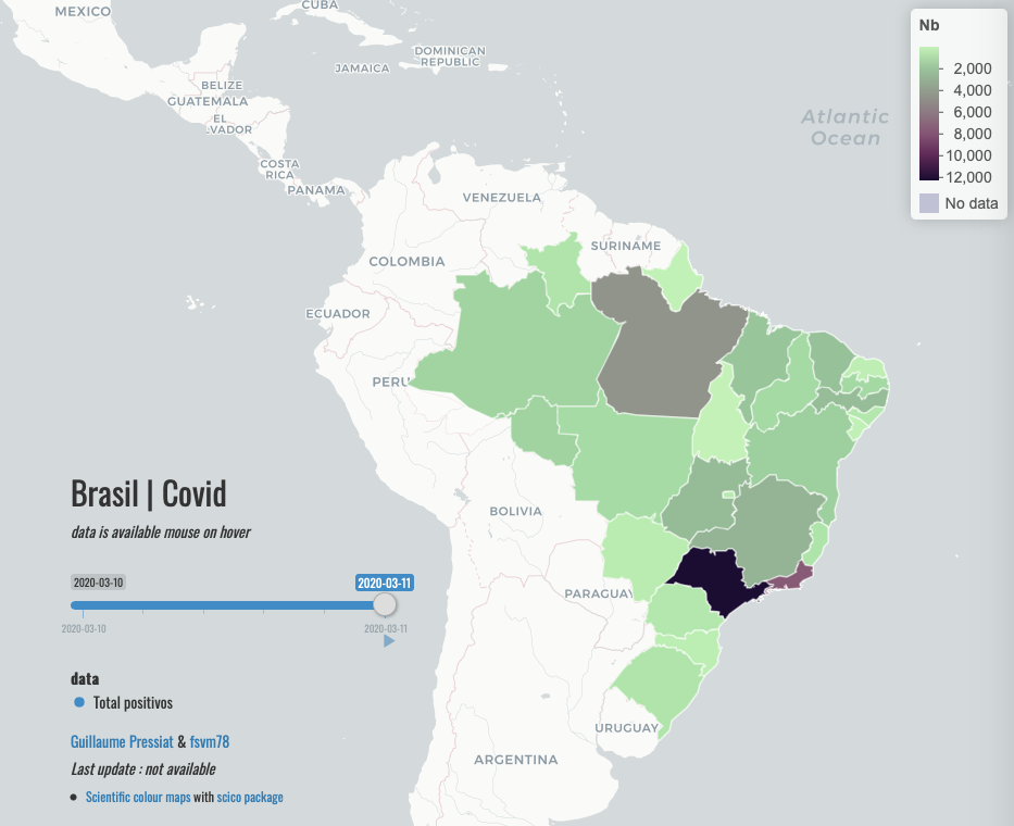
Code is here : https://github.com/GuillaumePressiat/covidbrasil

Not what you want (map on unidades da federação, not municipios) but time animation works.

Hope it helps.

Otherwise I see that in you dataset.csv, data are always the same for 10/03 and 11/03.

Hi, GuillaumePressiat,

with your help in simplifying the geojson, I am now able to make it fast. Thanks! (this really work) and I really appreciate the work you have done which I see it as a way to give more awareness during the COVID season. Respect!
While you are adding authentication on it which is another really cool feature! I feel astonished how you learned about this can be achieved by Shiny (through documentation? maybe).
As my first R project (new to R). basically learn the whole thing about shiny here and from the documentation. Thanks, I have already see you as a great teacher.

I am considering adding more features on this map.
An example which makes great sense for me is a map from:
https://coronavirus.1point3acres.com/en

I thought some great ideas can be found out when you explore this info site in design and make this app more attractive.

Hi @Halfbakedpanda,

Thanks for the feedback.

In case you haven't seen it : many shiny apps are collected here : https://www.statsandr.com/blog/top-r-resources-on-covid-19-coronavirus/ with open source code

Hi @GuillaumePressiat! I've been terrified these past few weeks and ended up not giving a return. Much work! Follow the code I made. I am grateful because I learned almost everything here and in the tutorials for shiny and leaflet. I am also improving in general in r (I am new), I have worked a lot in the analysis of scientific data. If my article is accepted I will make a special thanks to your help !!!

I am still trying to solve some problems with my code due to the size of the shapefile and the need to assess the level of the municipalities. I used Qgis to simplify my shapefile and now the app works better. If you have any more tips, thank you in advance!

https://drive.google.com/file/d/17D2CDQmyzoafQtf5n0DMOaw1b8Z3Tn5C/view?usp=sharing