Last active
April 11, 2024 07:24
-
-
Save ahwillia/2941fb64e8bfe999c66291257601dfb4 to your computer and use it in GitHub Desktop.
Linear Regression with a circular dependent variable
This file contains bidirectional Unicode text that may be interpreted or compiled differently than what appears below. To review, open the file in an editor that reveals hidden Unicode characters.
Learn more about bidirectional Unicode characters
| # The MIT License (MIT) | |
| # | |
| # Copyright (c) Alex H. Williams | |
| # | |
| # Permission is hereby granted, free of charge, to any person obtaining a copy of this software and associated documentation | |
| # files (the "Software"), to deal in the Software without restriction, including without limitation the rights to use, copy, | |
| # modify, merge, publish, distribute, sublicense, and/or sell copies of the Software, and to permit persons to whom the | |
| # Software is furnished to do so, subject to the following conditions: | |
| # | |
| # The above copyright notice and this permission notice shall be included in all copies or substantial portions of the | |
| # Software. | |
| # | |
| # THE SOFTWARE IS PROVIDED "AS IS", WITHOUT WARRANTY OF ANY KIND, EXPRESS OR IMPLIED, INCLUDING BUT NOT LIMITED TO THE | |
| # WARRANTIES OF MERCHANTABILITY, FITNESS FOR A PARTICULAR PURPOSE AND NONINFRINGEMENT. IN NO EVENT SHALL THE AUTHORS OR | |
| # COPYRIGHT HOLDERS BE LIABLE FOR ANY CLAIM, DAMAGES OR OTHER LIABILITY, WHETHER IN AN ACTION OF CONTRACT, TORT OR OTHERWISE, | |
| # ARISING FROM, OUT OF OR IN CONNECTION WITH THE SOFTWARE OR THE USE OR OTHER DEALINGS IN THE SOFTWARE. | |
| import numpy as np | |
| import matplotlib.pyplot as plt | |
| import scipy.stats | |
| normcdf = scipy.stats.norm.cdf | |
| normpdf = scipy.stats.norm.pdf | |
| from scipy.linalg import cho_factor, cho_solve | |
| from sklearn.base import BaseEstimator | |
| class CircularRegression(BaseEstimator): | |
| """ | |
| Reference | |
| --------- | |
| Brett Presnell, Scott P. Morrison and Ramon C. Littell (1998). "Projected Multivariate | |
| Linear Models for Directional Data". Journal of the American Statistical Association, | |
| Vol. 93, No. 443. https://www.jstor.org/stable/2669850 | |
| Notes | |
| ----- | |
| Only works for univariate dependent variable. | |
| """ | |
| def __init__(self, alpha=0.0, tol=1e-5, max_iter=100): | |
| """ | |
| Parameters | |
| ---------- | |
| alpha : float | |
| Regularization parameter | |
| tol : float | |
| Convergence criterion for EM algorithm | |
| max_iter : int | |
| Maximimum number of EM iterations. | |
| """ | |
| self.alpha = alpha | |
| self.tol = tol | |
| self.max_iter = max_iter | |
| def fit(self, X, y): | |
| """ | |
| Uses EM algorithm in Presnell et al. (1998). | |
| Parameters | |
| ---------- | |
| X : array | |
| Independent variables, has shape (n_timepoints x n_neurons) | |
| y : array | |
| Circular dependent variable, has shape (n_timepoints x 1), | |
| all data should lie on the interval [-pi, +pi]. | |
| """ | |
| # Convert 1d circular variable to 2d representation | |
| u = np.column_stack([np.sin(y), np.cos(y)]) | |
| # Randomly initialize weights. Ensure scaling does | |
| W = np.random.randn(X.shape[1], 2) | |
| W /= np.max(np.sum(X @ W, axis=1)) | |
| # Cache neuron x neuron gram matrix. This is used below | |
| # in the M-step to solve a linear least squares problem | |
| # in the form inv(XtX) @ XtY. Add regularization term to | |
| # the diagonal. | |
| XtX = X.T @ X | |
| XtX[np.diag_indices_from(XtX)] += self.alpha | |
| XtX = cho_factor(XtX) | |
| # Compute model prediction in 2d space, and projection onto | |
| # each observed u. | |
| XW = (X @ W) | |
| t = np.sum(u * XW, axis=1) | |
| tcdf = normcdf(t) | |
| tpdf = normpdf(t) | |
| self.log_like_hist_ = [ | |
| np.log(2 * np.pi) - | |
| 0.5 * np.mean(np.sum(XW * XW, axis=1), axis=0) + | |
| np.mean(np.log(1 + t * tcdf / tpdf)) | |
| ] | |
| for itr in range(self.max_iter): | |
| # E-step. | |
| m = t + (tcdf / (tpdf + t * tcdf)) | |
| XtY = X.T @ (m[:, None] * u) | |
| # M-step. | |
| W = cho_solve(XtX, XtY) | |
| # Recompute model prediction. | |
| XW = X @ W | |
| t = np.sum(u * XW, axis=1) | |
| tcdf = normcdf(t) | |
| tpdf = normpdf(t) | |
| # Store log-likelihood. | |
| self.log_like_hist_.append( | |
| np.log(2 * np.pi) - | |
| 0.5 * np.mean(np.sum(XW * XW, axis=1), axis=0) + | |
| np.mean(np.log(1 + t * tcdf / tpdf)) | |
| ) | |
| # Check convergence. | |
| if (self.log_like_hist_[-1] - self.log_like_hist_[-2]) < self.tol: | |
| break | |
| self.weights_ = W | |
| def predict(self, X): | |
| u_pred = X @ self.weights_ | |
| return np.arctan2(u_pred[:, 0], u_pred[:, 1]) | |
| def score(self, X, y): | |
| """ | |
| Returns 1 minus mean angular similarity between y and model prediction. | |
| score == 1 for perfect predictions | |
| score == 0 in expectation for random predictions | |
| score == -1 if predictions are off by 180 degrees. | |
| """ | |
| y_pred = self.predict(X) | |
| return np.mean(np.cos(y - y_pred)) | |
| if __name__ == "__main__": | |
| ## Synthetic time series data | |
| # Params | |
| n_obs = 3000 | |
| nX = 10 | |
| n_traversals = 10 | |
| noise_lev = 0.2 | |
| # Create time series where dependent variable, y moves around | |
| # the circle at constant velocity. | |
| _raw_y = np.linspace(0, 2 * n_traversals * np.pi, n_obs + 1)[:-1] | |
| y = _raw_y % (2 * np.pi) - np.pi | |
| # Create predictor variables | |
| X_locs = np.linspace(0, np.pi * 2, nX + 1)[:-1] | |
| X = np.array([scipy.stats.vonmises(loc=l, kappa=10.0).pdf(y) for l in X_locs]).T | |
| X += np.random.randn(n_obs, nX) * noise_lev | |
| ## Fit Model | |
| model = CircularRegression(max_iter=20) | |
| model.fit(X, y) | |
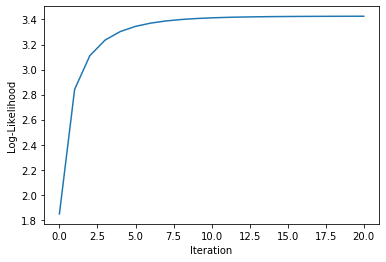
| plt.figure() | |
| plt.plot(model.log_like_hist_) | |
| plt.xlabel("Iteration") | |
| plt.ylabel("Log-Likelihood") | |
| ## Show Fit | |
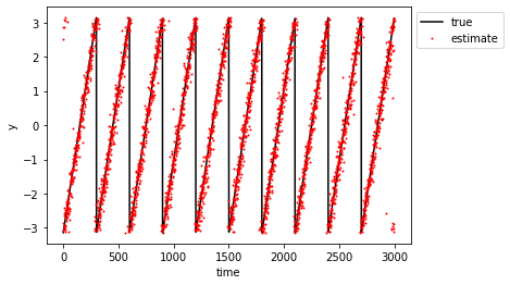
| plt.figure() | |
| plt.plot(y, "-k", label="true") | |
| plt.plot(model.predict(X), '.r', ms=2, label="estimate") | |
| plt.ylabel("y") | |
| plt.xlabel("time") | |
| plt.legend(bbox_to_anchor=(1,1,0,0)) | |
| plt.show() | |
| ## Cross Validation Demo | |
| from sklearn.model_selection import cross_val_score | |
| print(cross_val_score(CircularRegression(alpha=1.0), X, y, cv=5)) |
Sign up for free
to join this conversation on GitHub.
Already have an account?
Sign in to comment
Code Output
Cross-Validation Scores:
[0.95037565 0.95037833 0.94832496 0.95862434 0.94391777]Log-likelihood Learning Curve:
Model prediction (red) vs measurements (black):