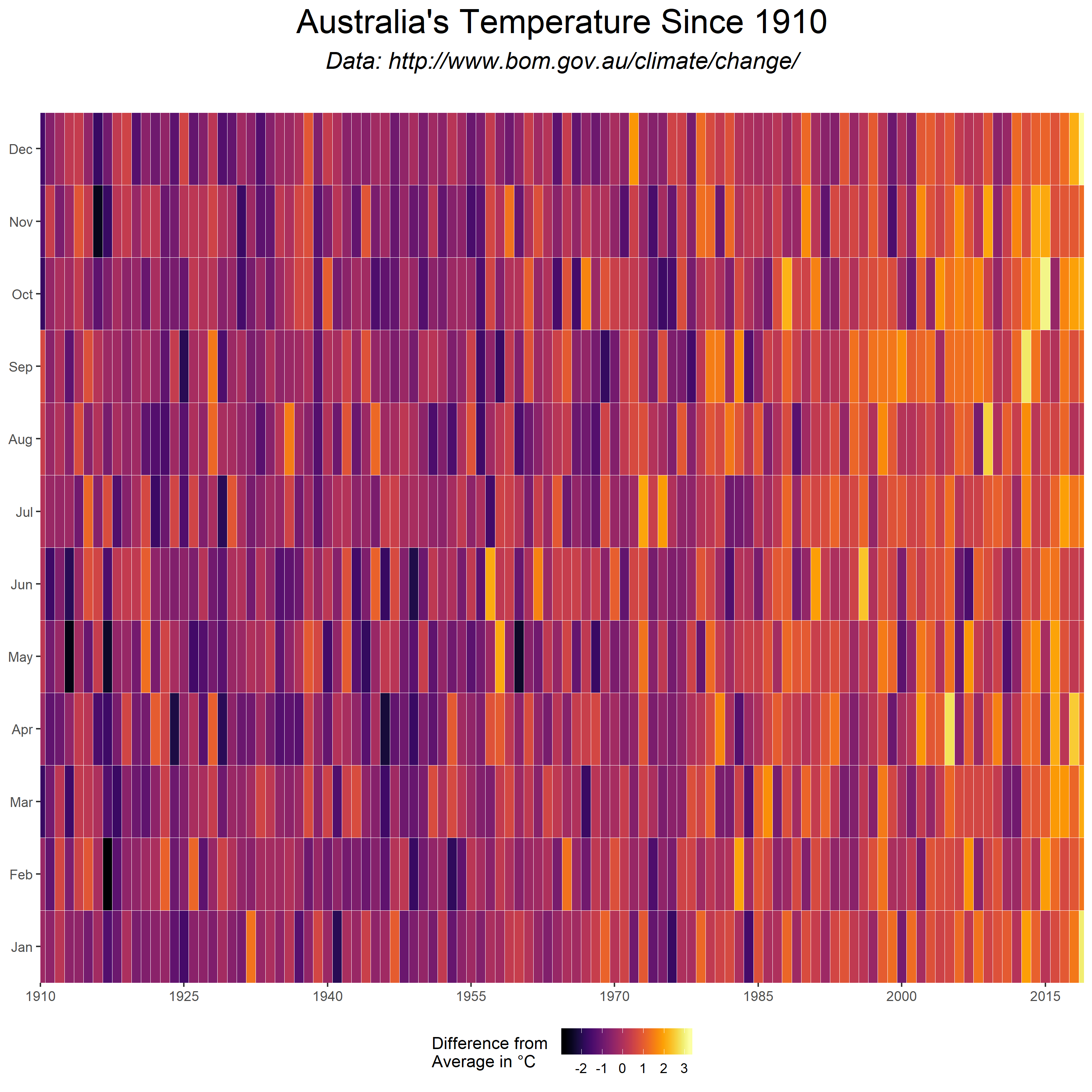
heatmap of australian temperature records. data from http://www.bom.gov.au/climate/change/#tabs=Tracker&tracker=timeseries

australiaheatmap.r

library(dplyr)
library(ggplot2)
library(tidyr)
library(viridis)
library(scales)
library(ggthemes)

aus<-read.csv("latest.txt",sep=",",header=FALSE)

names(aus)[1] <- "time"
names(aus)[2] <- "temp"

extract(aus, time, into = c("year", "month"), "^(\\d\\d\\d\\d)(\\d\\d).*$")

aus<-aus %>% 
  mutate(time = gsub('^(\\d\\d\\d\\d)(\\d\\d).*$', '\\1_\\2', time)) %>% 
  separate(time, into = c('year', 'month'), sep = '_')
  
aus$year <- as.numeric(as.character(aus$year))
aus$month <- as.numeric(as.character(aus$month))

dgr_fmt <- function(x, ...) {
        parse(text = paste(x, "", sep = ""))
}

a <- dgr_fmt(seq(1910,2019, by=15))
gg<-""
gg <- ggplot(aus, aes(x=year, y=month, fill=temp))
gg <- gg + geom_tile(color="white", size=0.1)
#gg <- gg + scale_colour_gradient2(name="Difference from \nAverage in °C",palette = "Spectral")
#gg <-gg + scale_fill_continuous_diverging()
#gg <-gg +scale_fill_distiller(palette = "Blue-Red 2")RdBu
#gg <- gg+ scale_colour_brewer(palette = "Spectral")
#gg <- gg + scale_fill_continuous_diverging("Blue-Red 3")
gg <- gg + scale_fill_viridis(name="Difference from \nAverage in °C",option="inferno")
plot.title = 'Australia\'s Temperature Since 1910'
plot.subtitle = 'Data: http://www.bom.gov.au/climate/change/'
gg <- gg + ggtitle(bquote(atop(.(plot.title), atop(italic(.(plot.subtitle)), ""))))
gg <- gg + labs(x=NULL, y=NULL)

gg <- gg +
        coord_cartesian(xlim = c(1910,2019)) +
        scale_x_continuous(expand = c(0, 0),breaks = seq(1910,2019, by=15), labels = a) +
        scale_y_continuous(expand = c(0, 0), 
                           breaks = c(1,2,3,4,5,6,7,8,9,10,11,12),
                           labels = c("Jan", "Feb", "Mar", "Apr",
                                      "May", "Jun", "Jul", "Aug", "Sep",
                                      "Oct", "Nov", "Dec"))


gg <- gg + theme(plot.title=element_text(hjust=0.5))
gg <- gg+ theme(plot.title = element_text(size=22))
gg <- gg +theme(plot.background=element_blank())
#gg <- gg +theme(panel.border = element_blank(),panel.grid.major = element_blank(), panel.grid.minor = element_blank())
          
gg <- gg+ theme(legend.position = "bottom")

ggsave("heatAus.png", width = 10, height = 10)

#Better red blue version has
library(RColorBrewer)
col_strip <- brewer.pal(11, "RdBu")
gg <- gg + scale_fill_gradientn(name="Difference from \nAverage in °C",colors = rev(col_strip)) #instead of gg <- gg + scale_fill_viridis

#water version
#as only anomolies for year 
gg <- ggplot(rain, aes(x=year,y=1, fill=rain))
#