Aerospike is a high performance distributed database, particularly well suited for real time transactional processing. It is aimed at institutions and use-cases that need high throughput ( 100k tps+), with low latency (95% completion in <1ms), while managing large amounts of data (Tb+) with 100% uptime, scalability and low cost.
Conceptually, Aerospike is most readily categorised as a key value database. In reality however it has a number of bespoke features that make it capable of supporting a much wider set of use cases. A good example is our document API which builds on our collection data types in order to provide JsonPath support for documents.
Another general use case we can consider is support for time series. The combination of buffered writes and efficient map operations allows us to optimise for both read and write of time series data. The Aerospike Time Series API leverages these features to provide a general purpose interface for efficient reading and writing of time series data at scale. Also included is a benchmarking tool allowing performance to be measured.
Time series data can be thought of as a sequence of observations associated with a given property of a single subject. An observation is a quantity comprising two elements - a timestamp and a value. A property is a measurable attribute such as speed, temperature, pressure or price. We can see then that examples of time series might be the speed of a given vehicle; temperature readings at a fixed location; pressures recorded by an industrial sensor or the price of a stock on a given exchange. In each case the series consists of the evolution of these properties over time.
A time series API in its most basic form needs to consist of
- A function allowing the writing of time series observations
- A function allowing the retrieval of time series observations
Additional conveniences might include
- The ability to write data in bulk (batch writes)
- The ability to query the data e.g. calculate the average, maximum or minimum.
The Aerospike Time Series API provides the above via the TimeSeriesClient object. The API is as follows
// Store a single data point for a named time series
void put(String timeSeriesName,DataPoint dataPoint);

// Store a batch of data points for a named time series
void put(String timeSeriesName, DataPoint[] dataPoints);

// Retrieve all data points observed between startDateTime and endDateTime for a named time series
DataPoint[] getPoints(String timeSeriesName,Date startDateTime, Date endDateTime);

// Retrieve the observation made at time dateTime for a named time series
DataPoint getPoint(String timeSeriesName,Date dateTime);

// Execute TimeSeriesClient.QueryOperation versus the observations recorded for a named time series
// recorded between startDateTime and endDateTime
// The operations may be any of COUNT, AVG, MAX, MIN or VOL (volatility)
double runQuery(String timeSeriesName, TimeSeriesClient.QueryOperation operation, Date fromDateTime, Date toDateTime);
A DataPoint is a simple object representing an observation and the time at which it was made, constructed as follows. The Java Date timestamp allows times to be specified to millisecond accuracy
DataPoint(Date dateTime, double value)The code example below shows us inserting a series of 24 temperature readings, taken in Trafalgar Square, London, on the 14th February 2022. We give the time series a meaningful and precise name by concatenating subject, property and units.
// Let's store some temperature readings taken in Trafalgar Square, London. Readings are Centigrade.
String timeSeriesName = "TrafalgarSquare-Temperature-Centigrade";
// The readings were taken on the 14th Feb, 2022
Date observationDate = new SimpleDateFormat("yyyy-MM-dd").parse("2022-02-14");
// ... and here they are
double[] hourlyTemperatureObservations =
	new double[]{2.7,2.3, 1.9, 1.8, 1.8, 1.7, 2.3, 3.2, 4.7, 5.4, 6.3, 7.7, 7.9, 9.9, 9.3,
               9.6, 9.7, 8.4, 7.4, 6.8, 5.5, 5.4, 4.3, 4.2};

// To store, create a time series client object. Requires AerospikeClient object and Aerospike namespace name
// new TimeSeriesClient(AerospikeClient asClient, String asNamespaceName)
TimeSeriesClient timeSeriesClient = new TimeSeriesClient(asClient,asNamespaceName);
// Insert our hourly temperature readings
for(int i=0;i<hourlyTemperatureObservations.length;i++){
  // The datapoint consists of the base date + the required number of hours
  DataPoint dataPoint = new DataPoint(
    Utilities.incrementDateUsingSeconds(observationDate,i * 3600),
    hourlyTemperatureObservations[i]);
  // Which we then 'put'
  timeSeriesClient.put(timeSeriesName,dataPoint);
}
As a diagnostic, we can get some basic information about the time series
TimeSeriesInfo timeSeriesInfo = TimeSeriesInfo.getTimeSeriesDetails(timeSeriesClient,timeSeriesName);
System.out.println(timeSeriesInfo);
which will give
Name : TrafalgarSquare-Temperature-Centigrade Start Date : 2022-02-14 00:00:00.000 End Date 2022-02-14 23:00:00.000 Data point count : 24
Another diagnostic allows the time series to be printed to the command line
timeSeriesClient.printTimeSeries(timeSeriesName);gives
Timestamp,Value
2022-02-14 00:00:00.000,2.70000
2022-02-14 01:00:00.000,2.30000
2022-02-14 02:00:00.000,1.90000
...
2022-02-14 22:00:00.000,4.30000
2022-02-14 23:00:00.000,4.20000
Finally we can run a basic query
System.out.println(
  String.format("Maximum temperature is %.3f",
                timeSeriesClient.runQuery(timeSeriesName,
                TimeSeriesClient.QueryOperation.MAX,
                timeSeriesInfo.getStartDateTime(),timeSeriesInfo.getEndDateTime())));
Maximum temperature is 9.900
Note we could alternatively have used the batch put operation, which 'puts' all the points in a single operation.
// Create an array of DataPoints
DataPoint[] dataPoints = new DataPoint[hourlyTemperatureObservations.length];
// Add our observations to the array
for (int i = 0; i < hourlyTemperatureObservations.length; i++) {
  // The datapoint consists of the base date + the required number of hours
  dataPoints[i] = new DataPoint(
    Utilities.incrementDateUsingSeconds(observationDate, i * 3600),
    hourlyTemperatureObservations[i]);
}
// Put the points in a single call
timeSeriesClient.put(timeSeriesName,dataPoints);There are two key implementation concepts to grasp. Firstly, rather than store each data point as a separate object, they are inserted into Aerospike maps. This minimises network traffic at write time (we only 'send' the new point) and allows large numbers of points to be potentially read at read time as they are encapsulated in a single object. It also helps minimise memory usage as Aerospike has a fixed (64 byte) cost for each object. Schematically, each time series object looks something like
{
	timestamp001 : value001,
	timestamp002 : value002,
	...
}
The maps must not grow to an indefinite extent, so the API ensures that each map will not grow beyond a specified maximum size. By default this limit is 1000 points, although this can be altered (see additional control). There is also a discussion in the README of the sizing and performance considerations associated with this setting.
The second implementation point follows on from the first. As there is a limit to the number of points that can be stored in a block, we need to have some mechanism for creating new blocks and keeping track of existing blocks for each time series. This is done, on a per time series basis, by maintaining an index of all blocks created. Conceptually this looks something like the following
{
	TimeSeriesName : "MyTimeSeries",
  ListOfDataBlocks : {
 		StartTimeForBlock1 : {EndTime: <lastTimeStampForBlock1>, EntryCount: <entriesInBlock1>},
 		StartTimeForBlock1 : {EndTime: <lastTimeStampForBlock1>, EntryCount: <entriesInBlock1>},
    ...
  }
}
The Time Series API ships with a benchmarking tool. Three modes of operation are provided - real time insert, batch insert and query. For details of how to download and run see the benchmarking section of the README.
As a simple example, let's insert 10 seconds of data for a single time series, with observations being made once per second.
./timeSeriesBenchmarker.sh -h <AEROSPIKE_HOST_IP> -n <AEROSPIKE_NAMESPACE> -m realTimeWrite -p 1 -c 1 -d 10Sample output
Aerospike Time Series Benchmarker running in real time insert mode

Updates per second : 1.000
Updates per second per time series : 1.000

Run time : 0 sec, Update count : 1, Current updates/sec : 1.029, Cumulative updates/sec : 1.027
Run time : 1 sec, Update count : 2, Current updates/sec : 1.000, Cumulative updates/sec : 1.013
Run time : 2 sec, Update count : 2, Current updates/sec : 0.000, Cumulative updates/sec : 0.672
...
Run time : 8 sec, Update count : 9, Current updates/sec : 1.000, Cumulative updates/sec : 1.003
Run time : 9 sec, Update count : 10, Current updates/sec : 1.000, Cumulative updates/sec : 1.003

Run Summary

Run time : 10 sec, Update count : 10, Cumulative updates/sec : 0.997
We can make use of another utility to see the output - ./timeSeriesReader.sh. This can be run for a named time series, or alternatively, will select a time series at random.
Here is sample output for our simple example
./timeSeriesReader.sh -h <AEROSPIKE_HOST_IP>  -n <AEROSPIKE_NAMESPACE>

Running TimeSeriesReader

No time series specified - selecting series AFNJFKSKDV

Name : AFNJFKSKDV Start Date : 2022-02-22 12:17:13.294 End Date 2022-02-22 12:17:23.185 Data point count : 11

Timestamp,Value
2022-02-22 12:17:13.294,97.37854
2022-02-22 12:17:14.247,97.34929
2022-02-22 12:17:15.263,97.33103
...
2022-02-22 12:17:22.212,97.31197
2022-02-22 12:17:23.185,97.29315
We can see that we have had sample points generated over a ten second period, with the series given a random name.
The benchmarker can be run at greater scale using the -c (time series count) flag. You may also wish to make use of -z (multi-thread) flag in order to achieve required throughput. The benchmarker will warn you if required throughput is not being achieved.
Another real time option is acceleration via the -a flag. This runs the simulation at an accelerated rate. So for instance if you wished to insert points every 30 seconds over a 1 hour period (120 points), you could shorten the time of the run by running using '-a 30'. This will 'speed up' the simulation by a factor of 30, so it will only take 120s. A higher number would also be possible. The benchmarker will indicate the actual update rates. For example
./timeSeriesBenchmarker.sh -h <AEROSPIKE_HOST>  -n <AEROSPIKE_NAMESPACE> -m realTimeWrite -c 5 -p 10 -a 10 -d 10
Aerospike Time Series Benchmarker running in real time insert mode

Updates per second : 5.000
Updates per second per time series : 1.000
A disadvantage of the 'real time' benchmarker is precisely that - the loading occurs in real time. You may wish to build your sample time series as quickly as possible. The batch insert mode is provided for this purpose.
In this mode, data points are loaded a block at a time - effectively as fast as the benchmarker will run. The invocation below, for example, will create 1000 sample series (-c flag), over a period of 1 year (-r flag), with 30 seconds between each observation.
./timeSeriesBenchmarker.sh -h <AEROSPIKE_HOST_IP> -n <AEROSPIKE_NAMESPACE> -m batchInsert -c 10 -p 30 -r 1Y
./timeSeriesBenchmarker.sh -h $HOST  -n test  -m batchInsert -c 1000 -p 30 -r 1Y -z 100

Aerospike Time Series Benchmarker running in batch insert mode

Inserting 1051200 records per series for 1000 series, over a period of 31536000 seconds

Run time : 0 sec, Data point insert count : 0, Effective updates/sec : 0.000. Pct complete 0.000%
Run time : 1 sec, Data point insert count : 1046000, Effective updates/sec : 870216.306. Pct complete 0.100%
Run time : 2 sec, Data point insert count : 2568000, Effective updates/sec : 1146363.231. Pct complete 0.244%
Run time : 3 sec, Data point insert count : 4196000, Effective updates/sec : 1308796.007. Pct complete 0.399%
Run time : 4 sec, Data point insert count : 5806000, Effective updates/sec : 1372576.832. Pct complete 0.552%
...
Run time : 577 sec, Data point insert count : 1051077000, Effective updates/sec : 1820986.414. Pct complete 99.988%
Run time : 578 sec, Data point insert count : 1051158000, Effective updates/sec : 1817977.108. Pct complete 99.996%

Run Summary

Run time : 578 sec, Data point insert count : 1051200000, Effective updates/sec : 1816538.588. Pct complete 100.000%
Having two different methods for generating data now puts us in the position where we can consider query benchmarking. This is the third and final aspect of the benchmarking toolkit.
Query benchmarking can be invoked via the 'query' mode. We choose how long to run the benchmarker for (-d flag) and the number of threads to use (-z flag).
At runtime, the benchmarker scans the database to determine all time series available. Each iteration of the benchmarker selects a series at random and calculates the average value of the series. The necessitates pulling all data points for the series to the client side and doing the necessary calculation so it is a good test of the query capability. We can ensure the queries are consistent in terms of data point value by using the batch insert aspect of the benchmarker which ensures all series have the same number of data points.
Sample invocation and output
./timeSeriesBenchmarker.sh -h $HOST -n test -m query -z 1 -d 120

Aerospike Time Series Benchmarker running in query mode

Time series count : 1000, Average data point count per query 1051200

Run time : 0 sec, Query count : 0, Current queries/sec 0.000, Current latency 0.000s, Avg latency 0.000s, Cumulative queries/sec 0.000
Run time : 1 sec, Query count : 1, Current queries/sec 1.003, Current latency 0.604s, Avg latency 0.604s, Cumulative queries/sec 0.999
Run time : 2 sec, Query count : 3, Current queries/sec 2.002, Current latency 0.585s, Avg latency 0.591s, Cumulative queries/sec 1.499
Run time : 3 sec, Query count : 5, Current queries/sec 2.000, Current latency 0.515s, Avg latency 0.561s, Cumulative queries/sec 1.666
Run time : 4 sec, Query count : 7, Current queries/sec 2.000, Current latency 0.583s, Avg latency 0.567s, Cumulative queries/sec 1.750
...
Run time : 120 sec, Query count : 241, Current queries/sec 2.000, Current latency 0.471s, Avg latency 0.496s, Cumulative queries/sec 2.008

Run Summary

Run time : 120 sec, Query count : 242, Cumulative queries/sec 2.016, Avg latency 0.496s
The Aerospike Time Series API contains a realistic simulator, which is made use of by the Benchmarker.
Many time series over a short period at least, follow a Brownian Motion. The TimeSeriesSimulator allows this to be simulated. The idea is that if we look at the relative change in our observed value, then the expected mean change should be proportional to the time between observations and the expected variance should similarly be proportional to the period in question. Formally, let X(τ) be the observation of the subject property X at time τ. After a time t let the value of X be X(τ+t). The simulation distributes the value of (X(τ +t) - X(τ)) / X(τ) i.e. the relative change in X like a normal distribution with mean μt and variance σ2t.
(X(t + τ) - X(t)) / X(t) ~ N(μt,σ2t.)More detail is available at simulation but it is useful to see that the net effect of the above is to produce sample series such as the one shown below
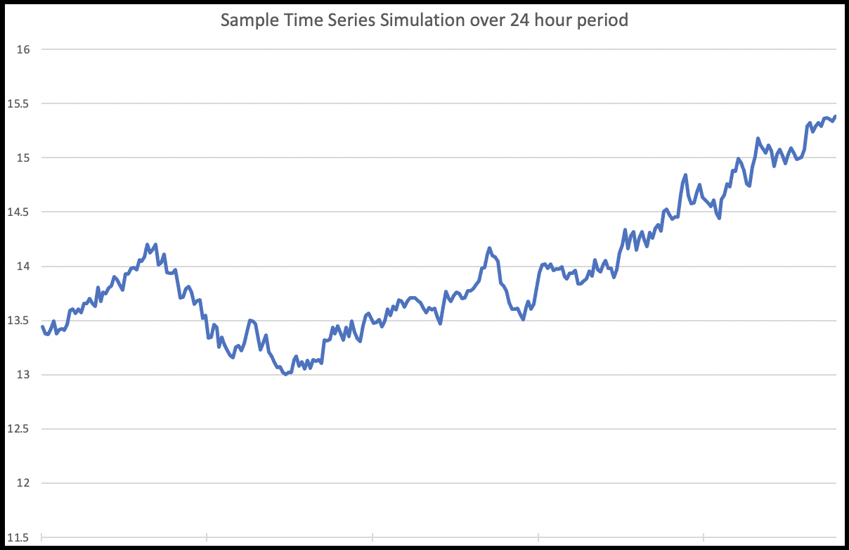
We can see it looks very much like the sort of graph we might see for a stock price.
More complex time series e.g. those seen for temperatures might be simulated by concatenating several series together, with different drifts and volatilities, allowing values to trend both up and down. Mean reverting series can be simulated by setting the drift to zero.
As a test, performance was examined on an Aerospike cluster deployed on 3 i3en.2xlarge AWS instances. This instance type was selected as the ACT rating of the drives is 300k, making the arithmetic simple.
In simple terms, this cluster can then support 100k (see Performance Considerations) * 1.5kbyte * 3 (number of instances) = 450mb of throughput.
We know our average write is ~8kb. We assume replication factor two for resilience purposes. Sustainable updates per second is then 450mb / 2 (replication factor) / 8kb = 28,000.
In practice a 50k update rate was easily sustained using the real time benchmarker. The reason the value is higher is that larger writes do not necessarily have a larger penalty than small writes. Also, the ACT rating guarantees operations are sub 1ms in latency 95% of the time, a guarantee not necessarily needed for time series inserts.
The cost of such a cluster would be $23k per year using on-demand pricing ($0.90 / hour / instance) or $16k per year ($0.61 / hour/ instance) if using a reserved pricing plan.
Queries retrieving 1 million points per query (1 year of observations every 30 seconds) were able to run at the rate of two per second, with end to end latency of ~0.5 seconds for a sustained period using the benchmarking tool.
At the time of writing, this is an initial release of this API. Further developments should be expected. Possible further iterations may include
- Data compression following the Gorilla approach which potentially allows data footprint to be reduced by 90%
- Labelling of data to support the easy retrieval of multiple properties for subjects. For example, several sensors may be attached to an industrial machine - it may be convenient to retrieve all this series simultaneously for analysis purposes.
- A REPL (read/eval/print/loop) capability to support interrogative analysis
The Time Series Client is available at Maven Central - aero-time-series-client. You can download directly or by adding the below to your pom.xml file.
<dependency>
  <groupId>io.github.aerospike-examples</groupId>
  <artifactId>aero-time-series-client</artifactId>
  <version>LATEST</version>
</dependency>