lognormal models in `brms`

brms_lognormal.md

library(brms)
library(bayestestR)

m <- brm(
  mpg ~ 1,
  family = lognormal(),
  data = mtcars,
  backend = "cmdstanr"
)

m_pars <- as.data.frame(m)
mu <- m_pars$b_Intercept
sigma <- m_pars$sigma

nd <- data.frame(whatever = NA)

linpred gives mu (log(median)), as expected:

posterior_linpred(m, newdata = nd) |> as.data.frame() |> 
  cbind(Median = mu) |> 
  exp() |> 
  describe_posterior()
#> Summary of Posterior Distribution
#> 
#> Parameter | Median |         95% CI |   pd |          ROPE | % in ROPE
#> ----------------------------------------------------------------------
#> V1        |  19.26 | [17.29, 21.40] | 100% | [-0.10, 0.10] |        0%
#> Median    |  19.26 | [17.29, 21.40] | 100% | [-0.10, 0.10] |        0%

But the epred knows how to get the actual expected values (exp(mu + (sigma^2)/2)):

posterior_epred(m, newdata = nd) |> as.data.frame() |> 
  cbind(Manual = exp(mu + (sigma^2)/2)) |> 
  describe_posterior()
#> Summary of Posterior Distribution
#> 
#> Parameter | Median |         95% CI |   pd |          ROPE | % in ROPE
#> ----------------------------------------------------------------------
#> V1        |  20.21 | [18.03, 22.56] | 100% | [-0.10, 0.10] |        0%
#> Manual    |  20.21 | [18.03, 22.56] | 100% | [-0.10, 0.10] |        0%

In other words, brms provides here more than just a syntactic-sugar-log-transformation.

Making a new lognromal family

In this one, the mean of Y (not log(Y)) is modeled.

Setup

lognormal2 <- custom_family(
  "lognormal2", 
  dpars = c("mu", "sigma"),
  links = c("identity", "log"), 
  lb = c(0, 0), 
  type = "real"
)

stan_funs <- "
  real lognormal2_lpdf(real Y, real mu, real sigma) {
    return lognormal_lpdf(Y | log(mu) - (sigma ^ 2)/2, sigma);
  }
"

stanvars <- stanvar(scode = stan_funs, block = "functions")

posterior_epred_lognormal2 <- function(prep) {
  brms::get_dpar(prep, "mu")
}

Fit

m2 <- brm(
  mpg ~ hp,
  family = lognormal2,
  data = mtcars,
  backend = "cmdstanr",
  stanvars = stanvars
)

ggpredict(m2, "hp") |> plot() # linear!

Looking at "true" mu parameters:

library(ggplot2)

nd <- data.frame(hp = with(mtcars, seq(min(hp), max(hp), length = 100)))

mu_ <- posterior_linpred(m2, newdata = nd, dpar = "mu")
sigma <- posterior_linpred(m2, newdata = nd, dpar = "sigma")
true_mu <- log(mu_) - (sigma ^ 2)/2

true_mu |> 
  as.data.frame() |> describe_posterior( test = NULL) |> 
  cbind(nd) |> 
  ggplot(aes(hp, Median)) +
  geom_ribbon(aes(ymin = CI_low, ymax = CI_high), alpha = 0.4) +
  geom_line() +
  labs(y = "mu")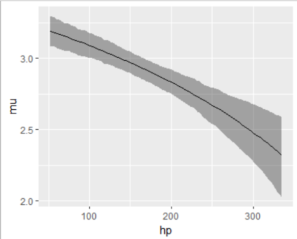

Alt, instead of modeling the expected value, we can model exp(mu) - the mu parameter on the response scale (a linear X to mu relationship).

stan_funs <- "
  real lognormal3_lpdf(real Y, real mu, real sigma) {
    return lognormal_lpdf(Y | log(mu), sigma);
  }
"