Spark is known as a fast general-purpose cluster-computing framework for processing big data. In this post, we’re going to cover how Spark works under the hood and the things you need to know to be able to effectively perform distributing machine learning using pyspark. The post assumes basic familiarity with Python and the concepts of machine learning like regression, gradient descent, etc.
Before we get into the nitty-gritty of what exactly Spark is and how it works, let’s first get familiar with a programming paradigm called MapReduce.
MapReduce is a programming model based on “split-apply-combine” strategy for performing parallel computations over data on a cluster of devices. A typical MapReduce program will express a parallelizable process in a series of map and reduce operations. Map operation maps the data to zero or more key-value pairs. And the reduce function takes in those key-value groups, and performs aggregation to get the result.
The thing to note is that the MapReduce execution framework takes care of handling the data, running the map and reduce operations in a highly optimized and parallelized manner on the cluster, resulting in a scalable solution.
MapReduce is not a magic spell that can perform every algorithmic task efficiently by running it concurrently on a cluster of machines. To be able to execute an algorithm concurrently on a cluster, we first need to decompose it into smaller tasks, and there are two approaches to go about it.
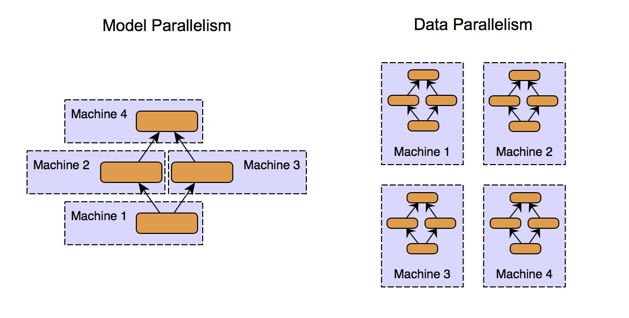
Model parallelism means functionally breaking down the logic into distinct and independent units, which can be later recomposed to get the results.
Data decomposition is a more obvious form of decomposition. Data is divided into chunks, and multiple machines perform the same computations on different chunks of data.
One instance where you can see both the functional and data decomposition in action is the training of an ensemble learning model like Random forest, which is conceptually a collection of decision trees. Decomposing the model into individual decision trees is "functional decomposition," and then further training an individual tree parallelly is data parallelism. It is also an example of what we can call as an Embarrassingly parallel task. Embarrassingly parallel tasks can be theoretically scaled infinitely by horizontally partitioning the data and adding more compute machines.
A MapReduce based framework implicitly exploits data-parallelism by partitioning the data and assigning concurrent processing tasks to the cluster nodes that can run independently. The term "independently" is important here, because if there’s a dependency between the tasks, i.e., tasks need to wait for other tasks to finish, the efficiency gets reduced. An example of such a case can be found most similar documents from a corpus, where we will have to evaluate every pair of documents together at least once to compute the similarity.
If the introduction until now doesn't make much sense to you, don't worry, we're about to dive deeper shortly!
The most common use case of MapReduce is querying Big Data for tasks like analytics. Google pioneered this technology for running queries on its massive datasets of web pages. Apache Hadoop is currently the most popular MapReduce framework, which was started as an open source project to implement the ideas discussed in the MapReduce paper published by Google.
As the framework matured and the need for efficiently handling big data grew, many companies started to leverage MapReduce using Hadoop. MapReduce kind of proved that cluster of machines working together is both faster and cheaper than a single really powerful machine. As time passed, multiple limitations of in Hadoop became apparent, and efforts were made to get around those limitations. The Spark project was launched as one such effort and is maintained by Apache. You can read this post for understanding the notable differences between Spark and Hadoop. That being said, spark performs better for iterative tasks where data can easily fit into the memory; that’s why it’s a good choice for performing machine learning.
Here’s how the high-level architecture of Spark looks like,
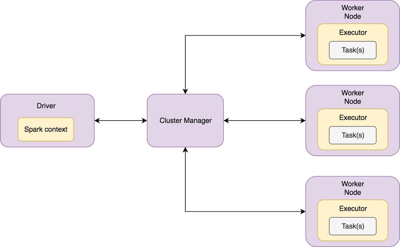
Spark has a master-slave (driver-worker) architecture. The driver is the central-coordinator in Spark. It connects to the Cluster manager for managing workers in which executors run. Driver and each of the executors run in their Java processes.
Drivers and executors in a Spark Application can run either locally or distributedly via a cluster manager. Spark local is a multi-threaded non-distributed runtime environment that doesn’t require a cluster manager. The drivers and the executors are spawned inside the same JVM in Spark local, and the degree of parallelism is determined by the number of threads specified at the time of instantiating the Spark Application. Local mode is suitable for testing and prototyping. The distributed mode, on the other hand, requires a cluster manager. A cluster manager is responsible for spawning executor processes on the workers. The workers communicate the resource availability (CPU and memory) to the cluster manager, and the cluster manager conveys this information to the driver whenever requested. Spark has a built-in cluster manager called Spark Standalone, and we can also plug other cluster managers like Hadoop YARN and Apache Mesos.
Spark is written in Scala and provides API at various levels of abstraction.
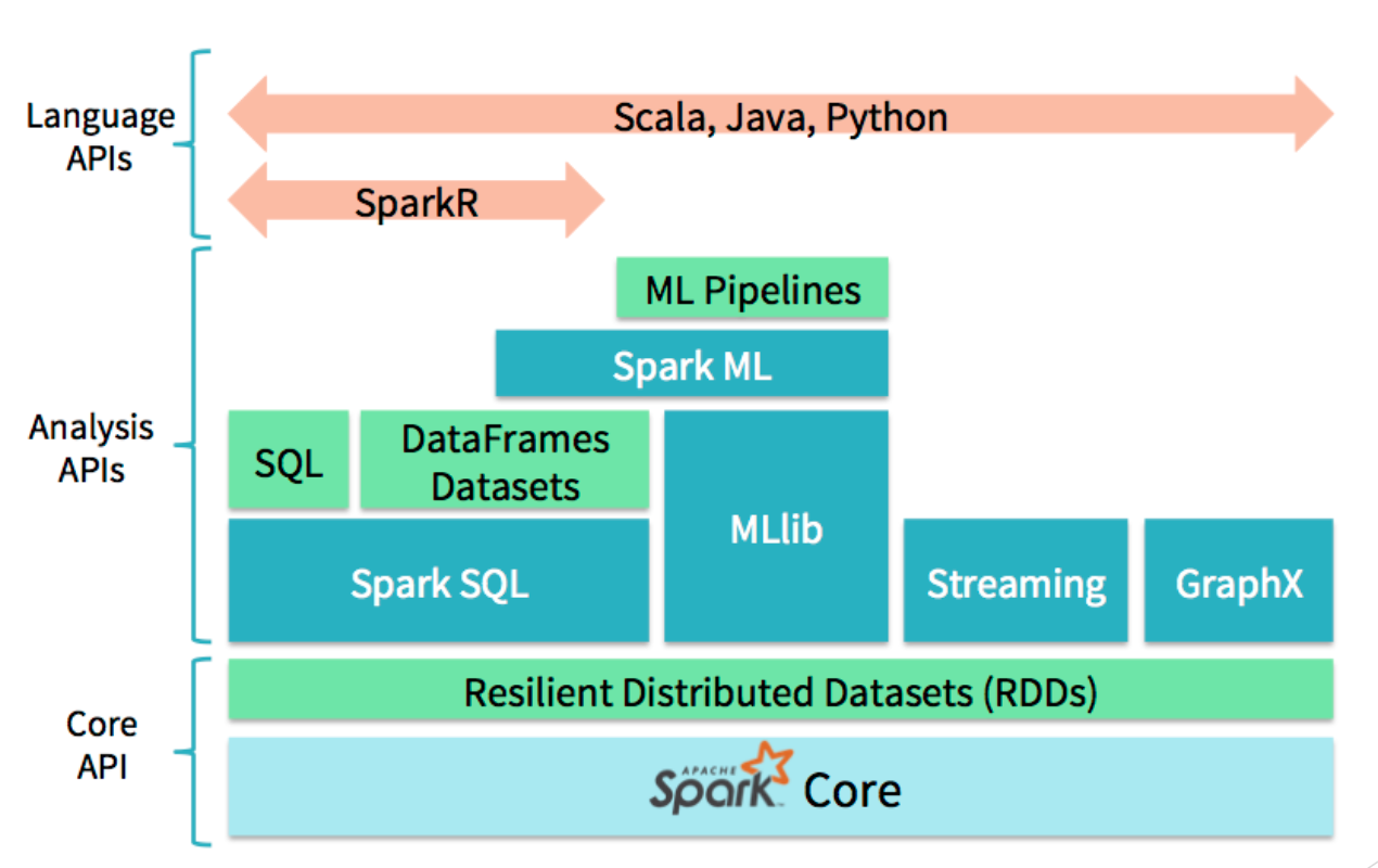
The core API is used to define configurations, create RDDs (basic data-structure of spark), and perform operations on it like map and reduce. There are libraries like GraphX, MLlib, SparkSQL, etc., that provide high-level APIs for analysis. And for versatility, Spark supports languages like Python, and R. pyspark is the Python language interface of Spark. Scala interface for spark could be a little bit faster than pyspark because it’s native. However, since python is a less verbose scripting language, has great dependency management, development process with pyspark might be faster.
To set up pyspark,
We have to first Install java if it's not already there on the machine, and then we can use pip to do the remaining work.
$ pip install pysparkpyspark also supports an interactive shell that we can use for quick prototyping. Just use the command pyspark to launch it, and make sure if everything is installed properly.
Let’s understand how MapReduce and Spark work by implementing a classic example of counting the words in a corpus (set of documents).
To launch spark and connect our app with spark, we need to instantiate a spark session. Here's how we are going to do that,
from pyspark.sql import SparkSession
app_name = "hello_world" # App name that'll be displayed on spark dashboard.
master = "local[*]"
spark = SparkSession.builder.appName(app_name).master(master).getOrCreate()
The local[*] parameter specifies to "Run Spark locally with as many worker threads as logical cores on your machine." getOrCreate will return an existing session or create one if it doesn't exist. Once the spark session is instantiated, you can go to http://localhost:4040 to see the spark dashboard.
Now let's say we have five documents in a corpus, and we have to count the occurrences of the words in the entire corpus. Here's how we'll be doing that,
# Defining our corpus, don't try to read it :p
corpus = [
  "Peter Piper picked a peck of pickled peppers",
  "A peck of pickled peppers Peter Piper picked",
  "If Peter Piper picked a peck of pickled peppers",
    "Where’s the peck of pickled peppers that Peter Piper picked",
    "peck picking"
]

# Creating an RDD
sc = spark.sparkContext
rdd = sc.parallelize(corpus)

>>> rdd
ParallelCollectionRDD[4685] at parallelize at PythonRDD.scala:195
>>> rdd.top(2)
['where’s the peck of pickled peppers that Peter Piper picked',
 'peter Piper picked a peck of pickled peppers']
You can think of spark.sparkContext as an entry point to anything dealing with the spark execution environment. In this snippet above, we defined our corpus and created an RDD for the corpus with SparkContext's parallelize method.
def emit_words(document):
        """
        Yields a tuple of the form (word, num_ocurrence) for
        every word in the docmuent.
        """
    for word in document.split():
          # Yielding 1 along with the word as a partial count
        # that we'll be aggregating later on.
        yield (word, 1)

word_emissions_rdd = rdd.flatMap(emit_words)
>>> word_emmisions_rdd
PythonRDD[4725] at RDD at PythonRDD.scala
>>> word_emissions_rdd.collect()
[('Peter', 1),
 ('Piper', 1),
 ('picked', 1),
 ('a', 1),
 ('peck', 1),
 ('of', 1),
 ('pickled', 1),
 ('peppers', 1),
 ('a', 1),
 ('peck', 1),
 ('of', 1),
 ('pickled', 1),
 ('peppers', 1),
 ('Peter', 1),
 ('Piper', 1),
 ('picked', 1),
 ('if', 1),
 ('Peter', 1),
 ('Piper', 1),
 ('picked', 1),
 ('a', 1),
 ('peck', 1),
 ('of', 1),
 ('pickled', 1),
 ('peppers', 1),
 ('where’s', 1),
 ('the', 1),
 ('peck', 1),
 ('of', 1),
 ('pickled', 1),
 ('peppers', 1),
 ('that', 1),
 ('Peter', 1),
 ('Piper', 1),
 ('picked', 1),
 ('peck', 1),
 ('picker', 1)]
Once we have our RDD object, we can perform operations on it to get the desired result. The first operation we are performing is map operation, i.e., mapping each document in our RDD to emit_words function, which in turns yields the words. You may notice that we've used flatMap in our example. The difference between a flatMap and map function is spark is that map "returns" exactly one value corresponding to the input, whereas flatMap can "yield" an arbitrary number of values.
word_counts_rdd = word_emissions_rdd.reduceByKey(lambda aggregated, current: aggregated + current)
>>> word_counts_rdd.collect()
[('of', 4),
 ('a', 3),
 ('where’s', 1),
 ('that', 1),
 ('picker', 1),
 ('pickled', 4),
 ('peck', 5),
 ('the', 1),
 ('picked', 4),
 ('peppers', 4),
 ('Peter', 4),
 ('Piper', 4),
 ('if', 1)]
After map is run, spark collects the outputs yielded by map, groups them based on the key, and performs the reduce operation. To get the word counts, we apply the reduceByKey operation to our word_emissions_rdd. The lambda function in our reduceByKey operation(lambda aggregated, current: aggregated + current) specifies spark to add the "current value" to the "aggregated value so far" during reduction, and finally, we get our word counts.
As mentioned earlier, RDD is the basic data structure of spark; it is what we perform all our operation on. Usually, the first step in every spark program is to load the data into an RDD. A few properties of RDD that we should be aware of are,
- Partitioned: An RDD is divided into multiple partitions. Different executors can concurrently perform computations on different partitions of RDD.
- Distributed: An RDD resides on multiple nodes across the cluster. A node need not have all the partitions of RDD.
- Resilient: If one of the nodes containing the partitions fails, spark has mechanisms to recover the lost data.
- Immutable: An RDD is a read-only object and cannot be modified. Transformation operation on RDDs generates a newer RDD.
In our example above, we created an RDD from a python list, but there a lot of different ways that you can use to create an RDD in spark. Spark provides APIs to access data from disk (textfile, csv, etc), Amazon S3, HDFS, Apache Cassandra, Apache HBase, Apache Hive, and lots of other data sources.
Spark records the sequence of operations applied to RDD in the form of Direct Acyclic Graph (called RDD lineage), so that they can be replayed in case of failure.
Two important components of SparkContext are the "DAGScheduler" and "TaskScheduler". The DAGScheduler transforms the logical execution plan (RDD lineage) to physical execution plan (TaskSets), one that's actually executed on workers. The physical execution plan is given to the TaskScheduler which is responsible for distributing the tasks to the executors through cluster manager.
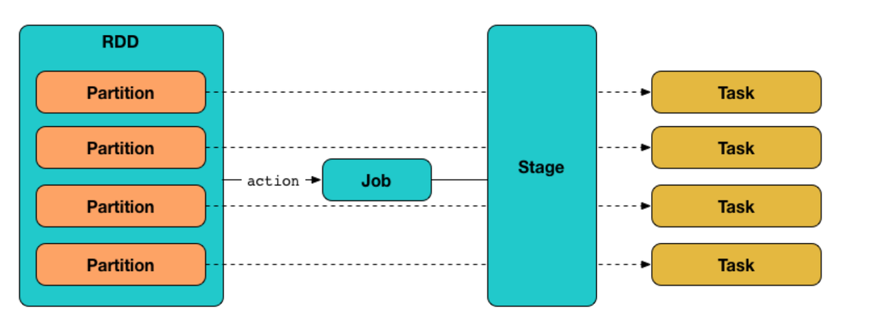
A Job in spark is the logical unit of execution, which is submitted to the DAGScheduler to compute the result of an action. A Stage is a physical unit of execution, it is a step in the physical execution plan. A stage consists of a set of parallel tasks (for different RDD partitions and executors). And tasks are the smallest physical units of execution responsible for computing a single partition of RDD.
There are two kinds of RDD operations in spark "transformations" and "actions". A transformation operation returns a new RDD, and an action returns a non-RDD object. The transformation operations are executed lazily in spark, i.e., The job is not submitted to the DAGScheduler for generating theTaskSets until an action is encountered in the RDD lineage.
Some commonly used transform operations in pyspark are
map,flatMap,mapValuesfilterdistinctunion,intersection,subtract,cartesian
Some commonly used actions in pyspark are
reduce,reduceByKeycollectcount,countByValuetake,takeOrderedtop
Lazy execution is the reason why printing the rdd in our example above just prints the object information and not the data (somewhat similar to generators in python). When the collect action is invoked, the operations are executed, and we get our data.
>>> word_emmisions_rdd
PythonRDD[4725] at RDD at PythonRDD.scala
>>> import sys
>>> sys.getsizeof(word_emmissions_rdd)
56
>>> sys.getsizeof(word_emissions_rdd.collect())
376Now that we understand "transformations and actions", "jobs, stages, and tasks", let's go back again to finding the most ocurring word in the corpus in one line of code,
# Getting the most ocurring word in one line
>>> rdd.flatMap(emit_words).reduceByKey(lambda x, y: x + y).sortBy(lambda x: -x[1]).collect()[0]
('peck', 5)
After flatMap is run, spark collects the outputs emitted by map, and performs optimized shuffling to distribute these emitted key-value pairs to the workers. Since reduceByKey aggregates the pairs based on the key, distribution happens in a such a way that all pairs corresponding to a particular key end up at the same worker. This means there's a "wide" dependency in the sense that spark has to
- Wait for all the executors performing map function to finish and yield their outputs.
- Shuffle the map output.
- Send these outputs to the workers based on the key.
Thus the above job (lines → words → per-word count → global word count → output) is performed in two stages in spark,
- Stage 1: lines → words → per-word count
- Stage 2: global word count → output
We can also use the higher level functions provided by pyspark like countByKey, takeOrdered, etc. to get similar results.
>>> rdd.flatMap(emit_words).reduceByKey(lambda x, y: x + y).takeOrdered(1, key=lambda x: -x[1])
[('peck', 5)]

>>> sorted(rdd.flatMap(emit_words).countByKey().items(), key = lambda x: x[1], reverse=True)[0]
('peck', 5)
Another cool feature of spark is the UI for visualizing the execution of jobs, which can be accessed at the address http://localhost:4040/
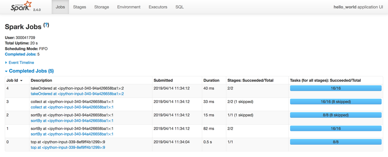
As you can observe, jobs are submitted only for action type operations. You can also see the DAGs,

and details at more granular level (stages and tasks)
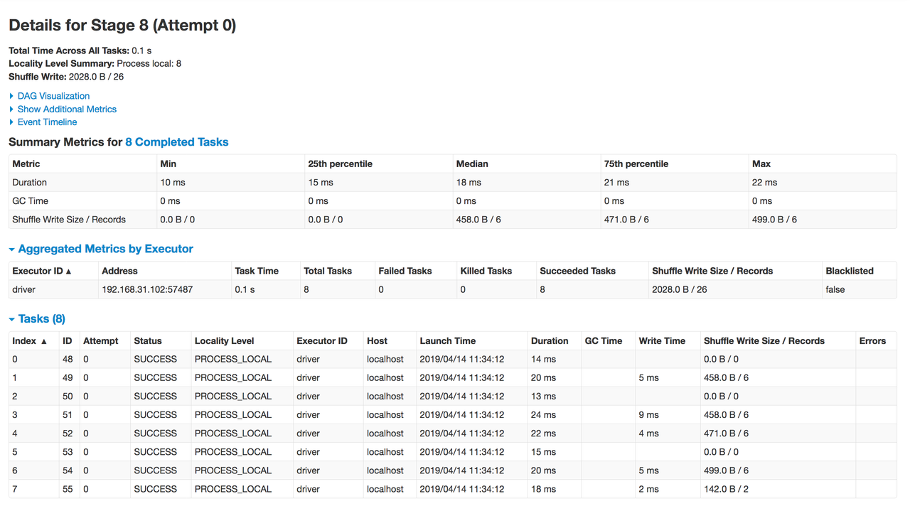
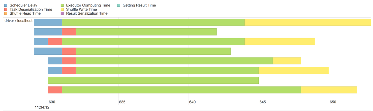
The dashboard can be handy for analyzing the performance, memory usage, and debugging the spark program.
Let's try to implement linear regression from scratch in pyspark. We'll be using the Wine Quality Data Set, but you can plug any other datasets too if you want. The wine quality dataset consists of 4800 instances having 12 attributes. We'll be predicting the wine quality using Linear regression (Ordinary Least Squares regression).
Let's download the data first,
$ wget -q -O data/dataset.csv http://archive.ics.uci.edu/ml/machine-learning-databases/wine-quality/winequality-white.csvdata_file = 'data/datset.csv'
header = !head -n 1 $data_file
FIELDS = re.sub('"', '', header[0]).split(';')
TARGET_FIELD = FIELDS[-1]
rdd = sc.textFile(data_file).filter(lambda x: x != header[0])
>>> FIELDS
['fixed acidity',
'volatile acidity',
'citric acid',
'residual sugar',
'chlorides',
'free sulfur dioxide',
'total sulfur dioxide',
'density',
'pH',
'sulphates',
'alcohol',
'quality']
>>> rdd.collect()[:5] # Check if it's loaded properly
['7;0.27;0.36;20.7;0.045;45;170;1.001;3;0.45;8.8;6',
'6.3;0.3;0.34;1.6;0.049;14;132;0.994;3.3;0.49;9.5;6',
'8.1;0.28;0.4;6.9;0.05;30;97;0.9951;3.26;0.44;10.1;6',
'7.2;0.23;0.32;8.5;0.058;47;186;0.9956;3.19;0.4;9.9;6',
'7.2;0.23;0.32;8.5;0.058;47;186;0.9956;3.19;0.4;9.9;6']The filter operation is used to restrict the records in the RDD. It takes in a function that returns a boolean, in our case we're using it to remove the header row from the RDD.
The attribute values in the rows are separated by ; , and the last attribute value corresponds to our target variable (the wine quality). Let's parse them using the map operation.
def parse_line(line):
    delimiter = ';'
    # split and convert to numpy array
    fields = np.array(line.split(delimiter), dtype = 'float')
    features, target_variable = fields[:-1], fields[-1]
    # emit tuple of features and targe-variable
    return(features, target_variable)

rdd = rdd.map(parse_line)

>>> rdd.collect()[:5]
[(array([7.000e+00, 2.700e-01, 3.600e-01, 2.070e+01, 4.500e-02, 4.500e+01,
         1.700e+02, 1.001e+00, 3.000e+00, 4.500e-01, 8.800e+00]), 6.0),
 (array([6.30e+00, 3.00e-01, 3.40e-01, 1.60e+00, 4.90e-02, 1.40e+01,
         1.32e+02, 9.94e-01, 3.30e+00, 4.90e-01, 9.50e+00]), 6.0),
 (array([8.100e+00, 2.800e-01, 4.000e-01, 6.900e+00, 5.000e-02, 3.000e+01,
         9.700e+01, 9.951e-01, 3.260e+00, 4.400e-01, 1.010e+01]), 6.0),
 (array([7.200e+00, 2.300e-01, 3.200e-01, 8.500e+00, 5.800e-02, 4.700e+01,
         1.860e+02, 9.956e-01, 3.190e+00, 4.000e-01, 9.900e+00]), 6.0),
 (array([7.200e+00, 2.300e-01, 3.200e-01, 8.500e+00, 5.800e-02, 4.700e+01,
1.860e+02, 9.956e-01, 3.190e+00, 4.000e-01, 9.900e+00]), 6.0)]Let's split the data into training and testing sets.
TRAIN_TEST_SPLIT = 0.8
train_rdd, test_rdd = rdd.randomSplit([TRAIN_TEST_SPLIT, 1 - TRAIN_TEST_SPLIT], seed = 1)
We've used the randomSplit operation to split the dataset 80-20 into train and test sets.
Every regression task usually involves some Exploratory Data Analysis to examine basic statistics of the attributes like mean, median, range, and variance. The intent is to find the features that have a linear relationship with the target variable and are not highly correlated.
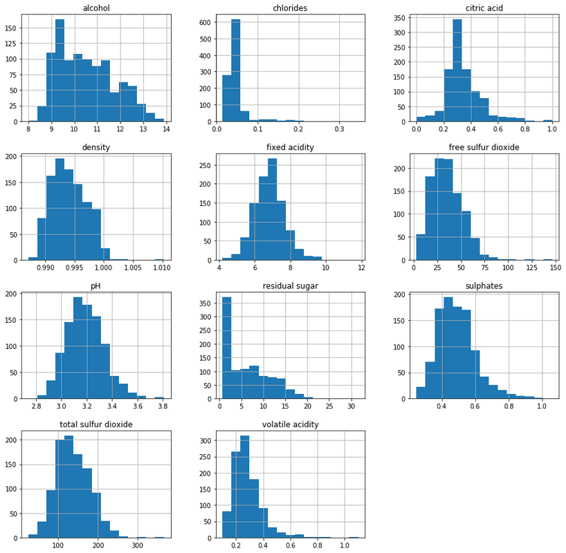
Let's first see how the distribution of our feature values looks like using histograms.
import pandas as pd

sample = np.array(train_rdd.map(lambda x: np.append(x[0], [x[1]]))
                                .takeSample(False, 1000))
sample_df = pd.DataFrame(np.array(sample), columns = FIELDS)
sample_df[FIELDS[:-1]].hist(figsize=(15,15), bins=15)
plt.show()
We've sampled 1000 records using the takeSample operation, constructed a pandas data frame, and plotted the histogram.
To check for the linear relationship, let's draw the box-plots for every feature with wine quality.
# Using seaborn to plot the boxplots
import seaborn as sns

fig, ax_grid = plt.subplots(4, 3, figsize=(15,15))
y = sample_df[TARGET_FIELD]
for idx, feature in enumerate(FIELDS[:-1]):
    x = sample_df[feature]
    # Adding some formatting magic so that it fist into a 3x3 grid
    sns.boxplot(x, y, ax=ax_grid[idx//3][idx%3], orient='h', linewidth=.5)
    ax_grid[idx//3][idx%3].invert_yaxis()
fig.suptitle(f"Individual Features vs {TARGET_FIELD}", fontsize=15, y=0.9)
plt.show()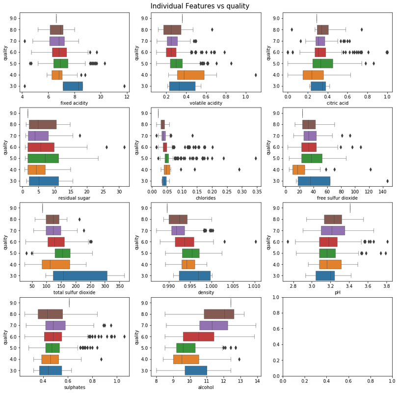
Let's check for highly correlated features by visualizing the correlation matrix with heatmap.
corr = sample_df[FIELDS[:-1]].corr()
fig, ax = plt.subplots(figsize=(11, 9))
mask = np.zeros_like(corr, dtype=np.bool)
mask[np.triu_indices_from(mask)] = True
cmap = sns.diverging_palette(240, 10, as_cmap=True)
sns.heatmap(corr, mask=mask, cmap=cmap, center=0, linewidths=.5)
plt.title("Correlations between features.")
plt.show()

There are a lot of observations from these plots that you can use to reduce the feature set. For example, the features color, chlorides, volatile acidity are positively correlated amongst each other and can be combined. What all features to remove is left as an exercise to the reader; you can use map to remove the features. We can also use filter operation to remove the outliers during EDA.
Let us now define a model that will predict the mean value of the target variable for every input. This will serve as our baseline, and we obviously want to do better than this.
mean_target_value = train_rdd.map(lambda x: x[1]).mean()

BASELINE = np.append([mean_target_value], np.zeros(len(train_rdd.take(1)[0][0]), dtype=np.float64))

>>> mean_target_value
5.8726065866734745

>>> BASELINE
[5.87260659 0.         0.         0.         0.         0.
 0.         0.         0.         0.         0.         0.        ]
np.zeros(len(train_rdd.take(1)[0][0]) is used for initialising weights (coefficients) corresponding to the features as zero. We append the bias term to the weights, and initialize the bias to mean value of the target variable. Now let's calculate the loss values for our baseline model.
We're going to use Ordinary Least Squares loss in our model.
def squared_error(args):
    label, prediction = args[0], args[1]
    return (label - prediction)*(label - prediction)

def ols_loss(rdd, weights):
    # Augmenting data for bias
    augmented_data = rdd.map(lambda x: (np.append([1.0], x[0]), x[1]))
    loss = augmented_data.map(lambda x: (np.dot(x[0], weights), x[1])).map(squared_error).mean()
    return np.sqrt(loss)
The data is augmented by appending 1 for the bias term in our baseline model. Then we compute the predicted value using the dot product, map it to the squared_error method, and finally, use the mean operation to get the MSE loss.
So here's the loss for our baseline model,
>>> ols_loss(train_rdd_parsed, BASELINE)
0.8832007562763831Now let's write the gradient descent algorithm that we'll be using to update the model weights during training. Here's the gradient descent equation as a quick refresher,
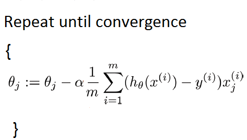
where "θ" represents weight for jth feature, m is the total number of observations, "h" is the function for predicting the target value using the weights (in case of linear regression, it is the dot product of weights and the input), "x" is the input record, and "y" is the actual target value corresponding to "x".
def gradient_descent_update(rdd, weights, lr=0.1):
    """
    Performs one gradient descent update. Returns updated coefficients,
    with bias at index 0.
    """
    # Add a feature of 1 corresponding to bias at index 0
    augmented_data = rdd.map(lambda x: (np.append([1.0], x[0].astype(np.float32, copy=False)), x[1]))

    # Compute the gradients; [h(x) - y] * x
    gradients = augmented_data.map(lambda x: (np.dot(x[0], weights), x[1], x[0])).map(lambda x: np.dot(x[0]- x[1], x[2])).cache()

    total_count = gradients.count()
    sum_of_gradients = gradients.sum()

    # Update weights using the gradients
    updated_weights = weights - lr * (1.0 / total_count) * sum_of_gradients
    return updated_weights
Notice the cache function called when computing the gradients? Whenever we have to perform multiple different operations on an RDD (count and sum in our case), it's better to cache it so that spark doesn't have to do redundant computations.
And here's our training logic.
def gradient_descent(train_rdd, test_rdd, initial_weights, num_iterations=20,
                    lr = 0.1):
    # tracking the history
    train_losses, test_losses, model_parameters = [], [], []

    model = initial_weights
    for idx in range(num_iterations):

        model = gradient_descent_update(rdd=train_rdd, weights=model)

        # Note: Computing losses after every iteration isn't required, but
        # we're computing it for visualization later.
        training_loss = ols_loss(train_rdd, model)
        test_loss = ols_loss(test_rdd, model)

        train_losses.append(training_loss)
        test_losses.append(test_loss)
        model_parameters.append(model)

        print("----------")
        print(f"STEP: {idx+1}")
        print(f"training loss: {training_loss}")
        print(f"test loss: {test_loss}")
        print(f"Model: {[round(w,3) for w in model]}")

return train_losses, test_losses, model_parametersLet's train our model!
initial_weights = BASELINE
start = time.time()
train_errors, test_errors, parameters = gradient_descent(train_rdd, test_rdd, train_losses, test_losses, model_parameters = gradient_descent(train_rdd, test_rdd, initial_weights, num_iterations = 50)
print(f"\n... trained {len(train_losses)} iterations in {time.time() - start} seconds")

# The output
# trained 50 iterations in 12.398797035217285 seconds
It took around 12 seconds to run 50 iterations. We've omitted the print output due to verbosity. Instead, we've collected the loss values and the model parameters after every iteration which we will visualize.
import matplotlib.pyplot as plt

def plot_error_curve(train_losses, test_losses, title = None):
    fig, ax = plt.subplots(1, 1, figsize = (16,8))
    x = list(range(len(train_losses)))[1:]
    ax.plot(x, train_losses[1:], 'k--', label='Training Loss')
    ax.plot(x, test_losses[1:], 'r--', label='Test Loss')
    ax.legend(loc='upper right', fontsize='x-large')
    plt.xlabel('Number of Iterations')
    plt.ylabel('Mean Squared Error')
    if title:
        plt.title(title)
    plt.show()

plot_error_curve(train_losses, test_losses, title = 'Ordinary Least Squares Regression' )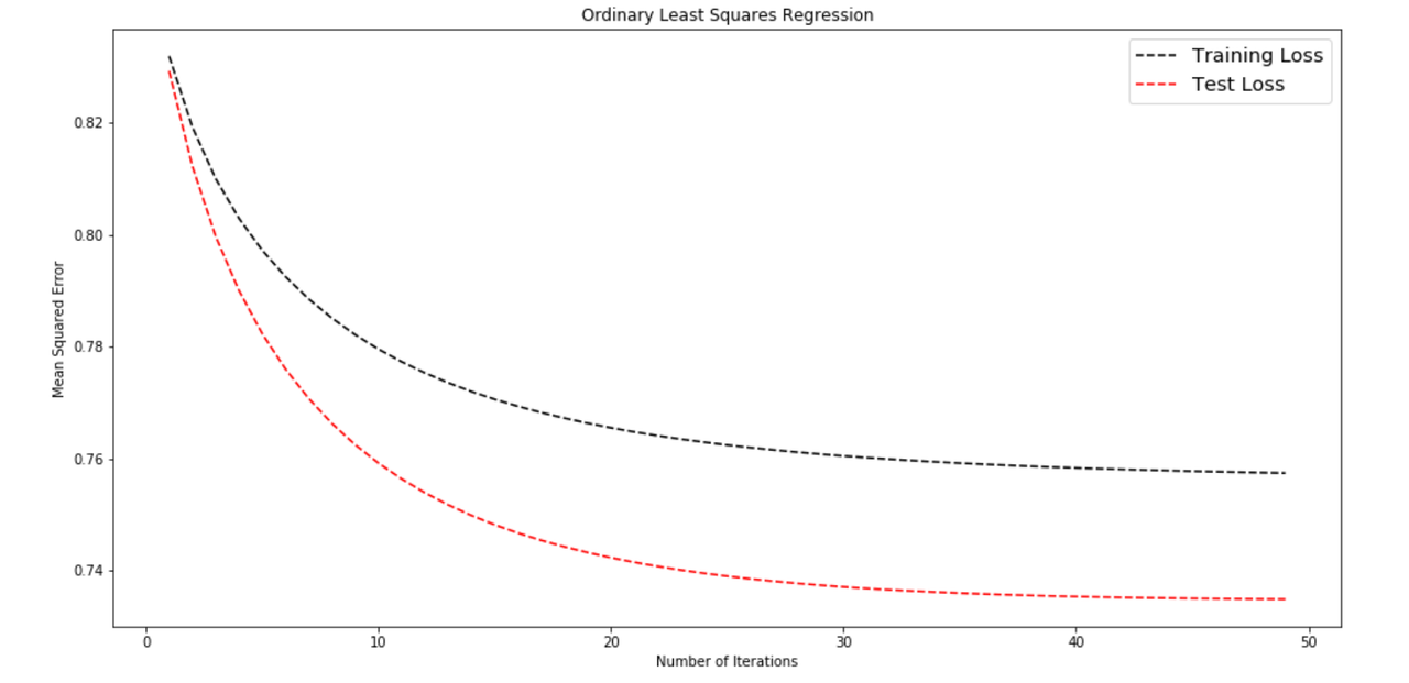
Notice the gap between training loss and test loss? That's due to overfitting, and we can reduce this with a technique called k-fold cross-validation. In the next section, we'll see how we can implement k-fold cross-validation, which is a slightly tricky task.
The conventional k-fold cross-validation process is something like this,
- Shuffle and then split the dataset into k splits
- For iteration
iin range1 to k- Hold out the ith split as test set
- Take the remaining splits as training sets
- Fit the model to the training set, evaluate score on the test set
- Retain the score and discard the model.
- Summarize the final scores.

Implementing the above algorithm as is in spark will lead to k-times increase in the execution time because we'll be performing the training of folds sequentially.
If we observe carefully, each record in k-fold cross-validation is used in the train set 1 time and used to train the model k-1 times. To perform it parallelly in spark, we can use k-models and update them simultaneously. In that way, we'll be making just one pass over the data records. You'll understand better with the actual implementation,
def k_residuals(record, models, split_num):
    """
    Compute the residuals for a data point given k different models. We emit
    a key to be able to track the residuals for a model number and train/test type.
    """
    # augment the data point with a bias term at index 0
    X = np.append([1.0], record[0])
    y = record[1]
    for model_num, weights in enumerate(models):
        if model_num == split_num:
            yield(f"{model_num}-test", (weights.dot(X) - y) ** 2)
        else:
            yield(f"{model_num}-train", (weights.dot(X) - y) ** 2)

def CV_loss(data_splits, models):
    """
    param data_splits: A list of k data splits.
    param model: A list of weights of k models.
    Compute the k-fold cross-validated test and train loss.
    """
    # compute k residuals for each data point (one for each model)
    # rdd to collect the residuals for diffferent splits
    partial_loss_rdd = sc.parallelize([])
    for split_num, rdd in enumerate(data_splits):
        residuals = rdd.flatMap(lambda x: k_residuals(x, models, split_num))
        # Add them to the existing residuals
        partial_loss_rdd = sc.union([partial_loss_rdd, residuals])

    # Reduce based on key to compute the train and test MSE for every model.
    loss = partial_loss_rdd.map(lambda x: (x[0], [x[1]])).reduceByKey(lambda x, y: x + y).map(lambda x: (x[0], np.mean(x[1]))).collect()

    # Check for the keys, and seperate training and testing losses.
    test_loss = np.mean([x[1] for x in loss if x[0].split('-')[1] == 'test'])
    training_loss = np.mean([x[1] for x in loss if x[0].split('-')[1] == 'train'])
    return training_loss, test_loss
The CV_loss method takes in a list of data-splits and model weights, iterates over the data splits, and computes residuals (Squared errors) for every record in the split using the k_residuals method. In the k_residuals method we compute the residuals for the data point against all the k models and label the ith residual as "test" (rest other are labeled "train"). We'll emit a key to track this. So one iteration will emit key-value pairs of the form [("1-test", 0.0123) ("2-train", 0.0345), …. ("k-train", kth_residual)]. These key-value pairs are collected in the partial_loss_rdd by using union operation to merge two RDDs. After that, we apply operations on partial_loss_rdd to compute the MSEs for train and test scenarios of every of the k models. Finally, we calculate the overall train and test loss by taking a mean across all the k models.
Note: This is perhaps the hardest logical part of the post to grasp that deals with intricacies of how to get things done with MapReduce paradigm. Half the battle of implementing any algorithm on spark is about representing it in the form of
mapandreducefunctions. It's all about taking the data, representing it in some form of key-value pairs by mapping, and then reducing those pairs to get the desired result.
After cross-validation loss, it's time to implement the cross-validation gradient descent step.
def partial_gradient(split_num, data_point, models):
    """
    Emit partial gradient for this data point for each model,
    except for the model corresponding to the split_num.
    """
    # augment the data point
    X = np.append([1.0], data_point[0])
    y = data_point[1]
    # emit partial gradients for each model with a counter for averaging later
    for model_num, weights in enumerate(models):
        if model_num != split_num:
              # Appending a 1 to the list to be able to compute
            # the total count during reduce step.
            yield (model_num, [(weights.dot(X) - y) * X, 1])

def CV_update(data_splits, models, lr = 0.1):
    """
    Compute gradients for k models given k corresponding data_splits.
    NOTE: The training set for model-k is all records EXCEPT those in the k-th split.
    """
    # compute partial gradient k-1 times for each fold
    partials_rdd = sc.parallelize([])
    for split_num, rdd in enumerate(data_splits):
        one_fold_partial_grads =  rdd.flatMap(lambda x: partial_gradient(split_num, x, models))
        partials_rdd = sc.union([partials_rdd, one_fold_partial_grads])

    # compute gradients by taking the average partialGrad for each fold
    # Note that the mapValues doesn't pass key at x[0] of the lambda.
    gradients = partials_rdd.reduceByKey(lambda a, b: (a[0] + b[0], a[1] + b[1]))\
                           .mapValues(lambda x: x[0]/x[1]) \
                           .map(lambda x: x[1]) \
                           .collect()

    # update all k models & return them in a list
    new_models = []
    for weights, grad in zip(models, gradients):
        new_model = weights - lr * grad
        new_models.append(new_model)
    return new_models
Notice that we've used mapValues instead of map. If your map method doesn't use the keys, then you can use mapValues to get some performance gain. Remember that the keys are not lost anywhere, and we're using them in the next map function (lambda x: x[1]) in the snippet above. Also, notice how we've used 1 in partial_gradient method to be able to compute the total count in reduceByKey operation of CV_update method (similar to what we did for word count).
Finally, comes our training logic...
def gradient_descent_with_cv(data_splits, initial_weights, lr=0.1, num_iterations = 5):
    """
    Train k models in parallel and track cross validated test/train loss.
    """
    # broadcast initial models (one for each fold).
    broadcasted_models = sc.broadcast([initial_weights] * len(data_splits))

    # initialize lists to track performance
    train_loss_0, test_loss_0 = CV_loss(data_splits, broadcasted_models.value)
    train_losses, test_losses, model_params = [train_loss_0], [test_loss_0], [initial_weights]

    # perform k gradient updates at a time (one for each fold)
    for step in range(num_iterations):
        new_models = CV_update(data_splits, broadcasted_models.value, lr)
        broadcasted_models = sc.broadcast(new_models)

        # log progress
        train_loss, test_loss = CV_loss(data_splits, broadcasted_models.value)
        train_losses.append(train_loss)
        test_losses.append(test_loss)
        model_params.append(new_models[0])

        print("-------------------")
        print(f"STEP {step}: ")
        print(f"model 1: {[round(w,4) for w in new_models[0]]}")
        print(f" train loss: {round(train_loss,4)}")
        print(f" test loss: {round(test_loss,4)}")

    return train_losses, test_losses, model_params
The training logic is similar to the vanilla gradient descent which we performed previously, except for the one thing, broadcasting. What is broadcasting and why do we need it? While invoking the CV_loss method, we pass a list of RDDs and a list of model weights. Then we iterate over the RDDs in CV_loss method and pass the same list of models to CV_update. Since operations on these different RDDs may end up on different executors, we'll have to ship a copy of the list of model-weights to every executor whenever the tasks are scheduled. But by broadcasting the list of model weights, spark will cache a distributed copy of the list on every worker, so that it doesn't get shipped every time, preventing the communication overhead.
k = 6
data_splits = rdd.randomSplit([1.0 / k] * k, seed = 1111)
initial_weights = BASELINE
start = time.time()
train_loss, test_loss, models = gradient_descent_with_cv(data_splits, initial_weights, num_iterations=50)
print(f"\n... trained {num_iterations} iterations in {time.time() - start} seconds")

# The output
# trained 50 iterations in 41.34121775627136 seconds
As we can observe, for 6-fold cross-validation, the training time increased by a factor of 3.5, although we still made only 1-pass over the data points. A few reasons for the increase in execution time are,
- We were computing residuals for 6 different models instead of one.
- The tasks are not entirely independent.
- I have only four cores in my CPU which limits the parallelization.
After all these limitations, we've performed pretty well. If we had gone with the sequential approach of performing 6-fold cross-validation, we'd have taken 6x more time.
Now let's see by plotting the error curve if we were able to narrow down the gap between test and training error values.
plot_error_curve(train_losses, test_losses, title = '6-fold Cross Validated Loss' )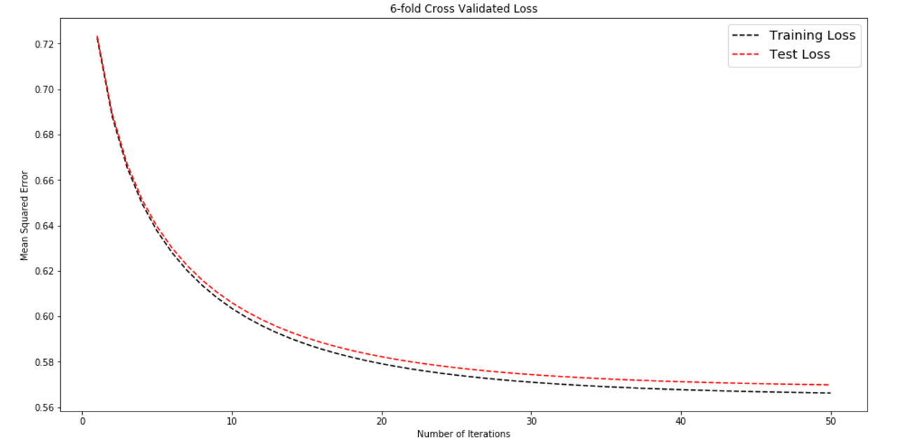
It seems like we've effectively reduced overfitting. The error values have also decreased.
Alright, now that we've learned things the hard way, let's explore some of the ways to make our lives easier,
Spark automatically partitions the RDDs without programmer's intervention. It tries to optimize its tasks scheduling considering the factors like existing data locations and the network distance of the node. In other words, it tries its best to get the optimal performance for your spark program. But there might be scenarios where tweaking the partition numbers, sizes, and scheme according to your application might give a decent performance boost. We recommend reading this post to understand how advanced partitioning can help in spark. Similarly, caching the RDDs in some scenarios, and keeping in mind of the execution plan can help you write the program in a more optimized way.
Spark has two built-in libraries spark.ml and spark.mllib for machine learning. These libraries provide a toolset to create pipelines of various machine learning related transformations on data. It includes common machine learning algorithms like classification, regression, clustering, etc. (here's the linear regression example using MLlib and SparkML), and APIs for tasks like dimensionality reduction, feature extraction, computing statistics, etc.
Why two libraries? MLlib provides APIs built on top of RDDs. To use its features, we've to work with data models like Vector, LabeledPoint, and Matrix. SparkML, on the other hand, provides a higher-level API built on dataframes, and is much easier to work with. MLlib is older and has more features, but all the features of MLlib are going to eventually migrate to SparkML, and it is going to be deprecated. You can read the official docs for the rationale behind this move.
Spark local is good for prototyping and testing, but to get real benefits of Spark we need to run our app on a cluster of machines. For executing spark application in the deployment environment, we need to set up the cluster of machines, and configure the cluster manager and the master. You can follow the instructions in this post for setting up a cluster from scratch.
Managing the cluster manually can be cumbersome, you can use cloud services like Amazon Web Services Elastic Map Reduce, Azure HDinsight, Google Dataproc provided by major cloud providers. These PaaS services can make your life easier by providing features like automatic scaling and configuration, easy deployment and monitoring, availability, and so on.
In this post, we understood the MapReduce paradigm and the internals of Apache Spark. By implementing gradient descent with k-fold cross-validation in pyspark, we covered the critical concepts that a programmer needs to know while implementing any machine learning algorithm in spark. And finally, we discovered the tools and services that can help us do production-scale Machine learning with pyspark.