chemlambda pred(3): graphviz dot file equivalent to mol file

README.md

Generating a graphviz dot file equivalent to the mol file of pred(3) in chemlambda v2: pred_3.mol (original name was erroneous)

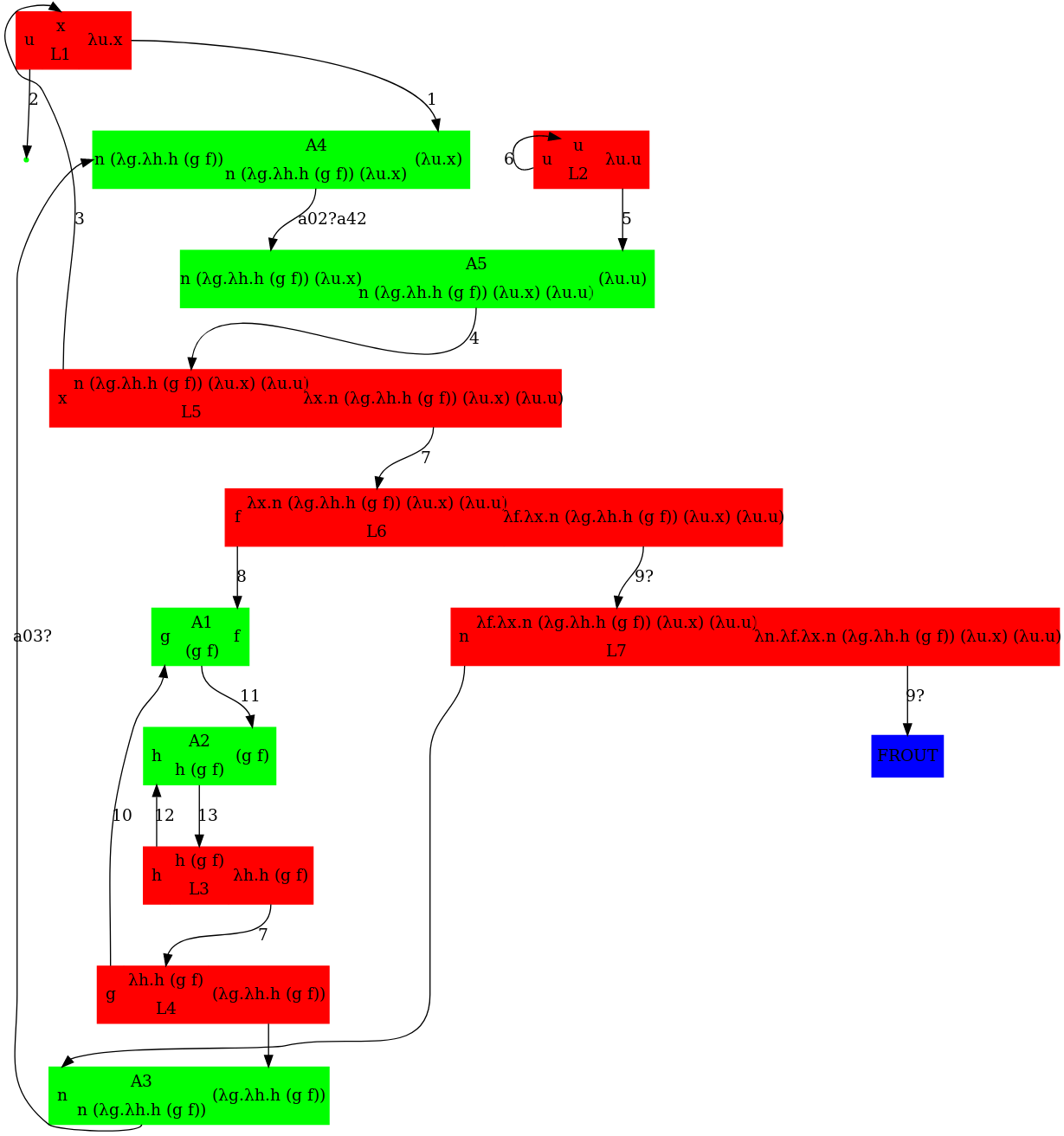
The lambda calculus expression for pred(3) (predecessor(3) == 2) is PRED := λn.λf.λx.n (λg.λh.h (g f)) (λu.x) (λu.u) (ref wikipedia)

Writing the above expression as nodes in a graph leads to the below graph. The corresponding dot file was written manually and available further below in this gist. An annotated version of pred_3.mol to help compare it to pred_3.dot is available further below in this gist.

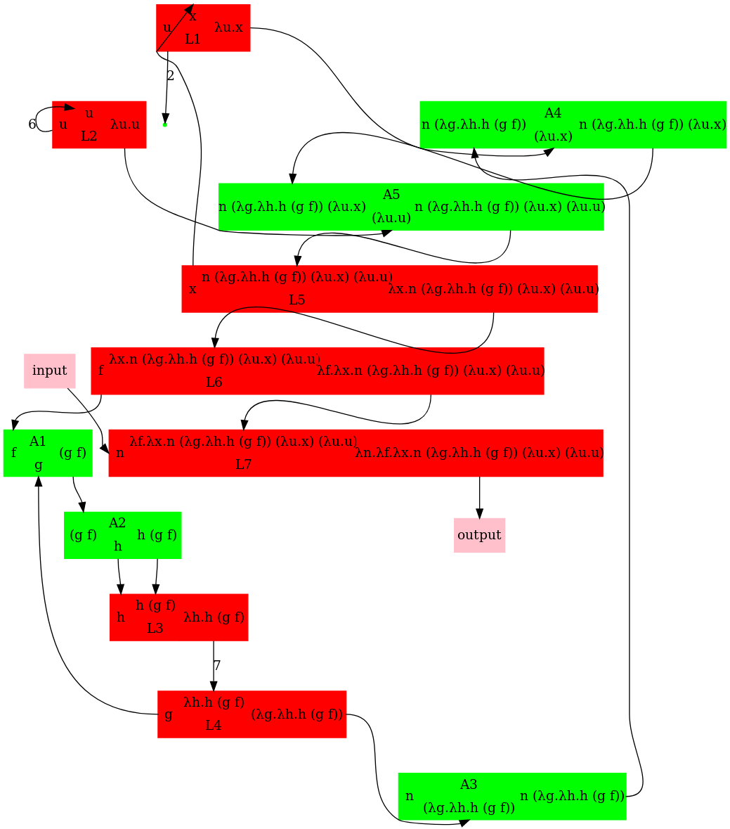
To generate the dot file automatically from lambda terms, check http://www.teamshadi.net/chemlambda-js/ (a fork from this jsfiddle ). Its current output for pred(3) matches with the manually specified graph below.

Version 4 (2019-04-11): shifted indeces back by 1 (e.g. L1 to L0) to match with the auto-generated graph from here

Compare the above graph to the chemlambda d3.js graph for pred_3.mol here

To experiment with graphviz, use http://www.webgraphviz.com/ or https://dreampuf.github.io/GraphvizOnline http://viz-js.com/

Notes:

• This work was prompted from chamlambda issue #6
• Older versions of graphs:

• Version 3 (2019-04-09):
• Version 2 (2019-04-07):

pred_3.dot

digraph G {
  rankdir = TB;

  // defaults for L
  node [shape=record, color=red, style=filled]; 
  L0 [label="<lo> u |{<mi> x|L0} | <ro> λu.x"];
  L1 [label="<lo> u |{<mi> u|L1} | <ro> λu.u"];
  L2 [label="<lo> h |{<mi> h (g f)|L2} | <ro> λh.h (g f)"];
  L3 [label="<lo> g |{<mi> λh.h (g f)|L3} | <ro> (λg.λh.h (g f))"];
  L4 [label="<lo> x |{<mi> n (λg.λh.h (g f)) (λu.x) (λu.u)|L4} | <ro> λx.n (λg.λh.h (g f)) (λu.x) (λu.u)"];
  L5 [label="<lo> f |{<mi> λx.n (λg.λh.h (g f)) (λu.x) (λu.u)|L5} | <ro> λf.λx.n (λg.λh.h (g f)) (λu.x) (λu.u)"];
  L6 [label="<lo> n |{<mi> λf.λx.n (λg.λh.h (g f)) (λu.x) (λu.u)|L6} | <ro> λn.λf.λx.n (λg.λh.h (g f)) (λu.x) (λu.u)"];

  // defaults for A
  node [shape=record, color=green, style=filled]; 
  A0 [label="<li> g |{A0|<mo> (g f)} | <ri> f"];
  A1 [label="<li> h |{A1|<mo> h (g f)} | <ri> (g f)"];
  A2 [label="<li> n |{A2|<mo> n (λg.λh.h (g f))} | <ri> (λg.λh.h (g f))"];
  A3 [label="<li> n (λg.λh.h (g f)) |{A3|<mo> n (λg.λh.h (g f)) (λu.x)} | <ri> (λu.x)"];
  A4 [label="<li> n (λg.λh.h (g f)) (λu.x) |{A4|<mo> n (λg.λh.h (g f)) (λu.x) (λu.u)} | <ri> (λu.u)"];

  // other
  T [ shape=point ]
  FROUT [ style=filled, color=blue ]
  //output [ style=filled, color=pink ]


  // aesthetics
//  {rank=same; L0 A4}
//  {rank=same; L1 L4}


  // build edges
  L0:lo -> T [ label=2 ]
  L1:lo -> L1:mi [ label=6 ]
  A1:mo -> L2:mi [ label=13 ]
  L2:ro -> L3:mi [ label=7 ]
  L3:ro -> A2:ri
  L6:lo -> A2:li
  A2:mo -> A3:li [ label="a03?" ]
  L0:ro -> A3:ri [ label=1 ]
  L1:ro -> A4:ri [ label=5 ]
  A3:mo -> A4:li [ label="a02?a42" ]
  A4:mo -> L4:mi [ label=4 ]
  L4:ro -> L5:mi [ label=7 ]

  // FIXME
  L5:ro -> L6:mi [ label="9?" ]
  // L5:ro -> FROUT [ label="9?" ]
  L6:ro -> FROUT [ label="9?" ]

  A0:mo -> A1:ri [ label=11 ]
  L2:lo -> A1:li [ label=12 ]

  L4:lo -> L0:mi [ label=3 ]
  L5:lo -> A0:ri [ label=8 ]
  L3:lo -> A0:li [ label=10 ]

  //L6:ro -> output
}


// https://en.wikipedia.org/wiki/Lambda_calculus
// PRED := λn.λf.λx.n (λg.λh.h (g f)) (λu.x) (λu.u)

pred_3.mol

L    3   2   1    3:x, 2:u1   L1
T    2            2:u1
L    6   6   5    6:u2
L    4   3   7    3:x         L5
L    7   8   9    8:f         L6
A   10   8  11    8:f, 10:g   A1
A   12  11  13                A2
L   13  12  14                L3
L   14  10 a43
A  a42   5   4                A5
A  a03   1 a02                A4!
FO a13 a11 a03
A  a11 a02 a12      
FO a43 a41 a13
A  a41 a12 a42                A4?


Not sure: L2, L4, L7?   A3, A4?

Many problems still.
(1) Arrow orientations wrong (ex. arrow from L2 to A3, corresponding to h)
(2) what is "input" and "output"?
(3) problems with port types. It's easy. The mol A a b c tells that:

• a is on port li
• b on port ri
• c on port mo

Same for FI a b c.

For L a b c you have

• a on port mi,
• b on port lo
• c on port ro

Same for FO and FOE.

For T a and FROUT a you have

• a on port mi

For FRIN a you have

• a on port mo

For Arrow a b you have

• a on port mi
• b on port mo

Any port variable appears at most twice in a port. If it appears exactly twice, it should appear once in one of the ports li, ri, mi, and once in one of the ports lo, eo, mo. It represents an arrow directed from a port lo, mo, mo, to a port li, ri, mi. If the variable appears only once, ten it is a free arrow. So if a appears once in a li, ri, mi port, then you have to add a FRIN a, otherwise it appears in a lo, ro, mo and you have to add a FROUT a. (this explains the types of ports for FRIN, frout and T)

(4) Why A1, A2, L7, etc? A, L, FI, FO, FOE, T, Arrow, FRIN and FROUT are types of nodes. Why concatenate a node type with a numbering of nodes?

Mind that the node numbering is not part of the fatgraph. In the mol notation you may take the node numbering as the number of line, but this is only because computers are as they are. The graph rewrites don't care about the order of lines in the mol file and they should not care about the numbering of the nodes.

Thanks @mbuliga for your corrections:

• Fixed ... Arrow orientations wrong (ex. arrow from L2 to A3, corresponding to h)
• what is "input" and "output"?
  • These are utility atoms that I added to see where the graph "starts/ends".
  • I understand now that it ends at "FROUT", am I mistaken?
• Fixed ... problems with port types. A a b c == A li ri mo, L a b c == L mi lo ro, ...
• Why A1, A2 ... without numbering
  • The reason I appended the numbers is just that it makes it easier to debug between the graphviz dot file and the graphical drawing
  • It also makes it easier to identify which row from the mol file I'm comparing with
  • Yes I agree that the numbering is irrelevant for the fatgraph and the rewrites

The above points you highlighted are fixed now. Do you mind checking again if I missed anything?
I'm sure that I am still missing something because I do not match 100% with the d3.js visualization of pred(3) that you have here. For example, I'm not sure where my L2, L4, L7? A3, A4? are on your d3.js graph. Also, the edges a02, a42, a03 from your mol file are not clear to me where they belong in my graph.

Thank you for the effort! Here is what I got after 2 hours of trying to understand pred_2.mol. The short message is that it is indeed PRED 3 but after 3 graphical beta rewrites. This is because pred_2.mol is part of experiments which led to chemlambda quines, see for example this description [1].

Further I shall use the rewrites from chemlambda as described in [2].

Let's start with some lambda terms

D = \g.\h.(h(gf))

PRED = \n.\f.\x.( (( (n D ) (\u.x) ) (\v.v)) )

3 = \y.\z.(y(y(yz)))

T = PRED 3

The term T is the lambda term which interests us. Let's see the mol file which is obtained from turning it into a "molecule".

Further I add the line number like this (1), at the beginning of the line, which identifies in your notation with the node number. At the end of the line I add info about whose node it is, like (\u.x). In order to obtain a valid mol file you have first to delete all line numbers and spaces before the node types, as well as all spaces and info after the last port variable.

(1) L 3 2 1 (\u. from \u.x from PRED)
(2) T 2 (u from \u.x does not occur elsewhere in PRED)
(3) L 6 6 5 (\v.v from PRED)
(4) L 4 3 7 (\x. from PRED)
(5) L 7 8 9 (\f. from PRED)
(6) A 10 8 11 (the application of g to f in D)
(7) A 12 11 13 (the application of h to gf in D)
(8) L 13 12 14 (\h. from D)
(9) L 14 10 a43 (\g. from D)
(10) A 19 5 4 (the application of (nD)(\u.x) to (\v.v) from PRED)
(11) A a03 22 a02 (the application yz from 3)
(12) FO a13 a11 a03 (2nd and 3rd occurrence of y in 3)
(13) A a11 a02 a12 (the application of y to (yz) in 3)
(14) FO 21 a41 a13 (1st occurrence of y and input to node (12) in 3)
(15) A a41 a12 a42 (1st application of y to y(yz) in 3)
(16) A 24 a43 17 (the application n to D in PRED)
(17) A 17 1 19 (the application (nD) to (\u.x) in PRED)
(18) L 18 21 16 (\y. from 3)
(19) L a42 22 18 (\z. from 3)
(20) L 9 24 23 (\n. from PRED)
(21) A 23 16 25 (the application of PRED to 3)

not figured in the mol (because my script add the FRIN and FROUT nodes if they are needed)

(22) FROUT 25 (the output, the term T)

The mol file has 21 lines, or 22 with the FROUT line, wich means that the molecule has 21 or 22 nodes with the FROUT node. The pred_2.mol has 15 lines, meaning it describes a molecule with 15 nodes, FROUT (or perhaps FRIN) excluded.

Why is it then claimed to be the chemlambda version of PRED 3? Because I already did some reductions. These are 3 (partial) beta reductions. The same is true for https://github.com/chorasimilarity/chemlambda-gui/blob/gh-pages/dynamic/mol/bigpred.mol which is the correspondent of PRED 28.

We start to reduce (graphically) this "molecule". There is a first beta rewrite which erases the nodes (20) and (21)

L 9 24 23, A 23 16 25 --> Arrow 16 24, Arrow 9 25

Then there are two COMB rewrites which eliminate the two Arrow nodes and renumber the edges: 24 --> 16 , 25 --> 9.

This can be seen as the lambda calculus beta rewrite

PRED 3 --> PRED[n=3]

and still the modified mol file represents exactly the term PRED[n=3]

(1) L 3 2 1 (\u. from \u.x from PRED[n=3])
(2) T 2 (u from \u.x does not occur elsewhere in PRED[n=3])
(3) L 6 6 5 (\v.v from PRED[n=3])
(4) L 4 3 7 (\x. from PRED[n=3])
(5) L 7 8 9 (\f. from PRED[n=3])
(6) A 10 8 11 (the application of g to f in D)
(7) A 12 11 13 (the application of h to gf in D)
(8) L 13 12 14 (\h. from D)
(9) L 14 10 a43 (\g. from D)
(10) A 19 5 4 (the application of (3 D)(\u.x) to (\v.v) from PRED[n=3])
(11) A a03 22 a02 (the application yz from 3)
(12) FO a13 a11 a03 (2nd and 3rd occurrence of y in 3)
(13) A a11 a02 a12 (the application of y to (yz) in 3)
(14) FO 21 a41 a13 (1st occurrence of y and input to node (12) in 3)
(15) A a41 a12 a42 (1st application of y to y(yz) in 3)
(16) A 16 a43 17 (the application 3 to D in PRED[n=3])
(17) A 17 1 19 (the application (3 D) to (\u.x) in PRED[n=3])
(18) L 18 21 16 (\y. from 3)
(19) L a42 22 18 (\z. from 3)

not figured

{22} FROUT 9 (the output, the term PRED[n=3])

We can perform two (graphical) beta rewrites and we obtain the mol file which is misleadingly named http://imar.ro/~mbuliga/pred_2.mol . In lambda calculus this corresponds almost to two beta rewrites in the sub-term (3 D) (\u.x). In lambda calculus this should lead to the subterm (3[y=D])[z=\u.x]. But in chemlambda, even if we do two beta rewrites, we end just before to replace the occurrences of y with copies of D.

Let's see this:

L 18 21 16, A 16 a43 17 --> Arrow a43 21, Arrow 18 17

The nodes (18) and (16) are eliminated and two COMB rewrites renumber the edges: 21 --> a43 , 17 --> 18. We get the mol file

(1) L 3 2 1 (\u. from \u.x )
(2) T 2 (u from \u.x does not occur elsewhere )
(3) L 6 6 5 (\v.v from ...)
(4) L 4 3 7 (\x. from ...)
(5) L 7 8 9 (\f. from ...)
(6) A 10 8 11 (the application of g to f in D)
(7) A 12 11 13 (the application of h to gf in D)
(8) L 13 12 14 (\h. from D)
(9) L 14 10 a43 (\g. from D)
(10) A 19 5 4 (the application of (3 D)(\u.x) to (\v.v) )
(11) A a03 22 a02 (the application (y=D)z from 3)
(12) FO a13 a11 a03 (2nd and 3rd occurrence of (y=D) in 3)
(13) A a11 a02 a12 (the application of (y=D) to ((y=D)z) in 3)
(14) FO a43 a41 a13 (1st occurrence of (y=D) and input to node (12) in 3)
(15) A a41 a12 a42 (1st application of (y=D) to (y=D)((y=D)z) in 3)
(17) A 18 1 19 (the application (3 D) to (\u.x) )
(19) L a42 22 18 (\z. from 3)

not figured

{22} FROUT 9 (the output)

This mol file contains the node (9) L 14 10 a43 whose output a43 is the input of the node (14) FO a43 a41 a12. This configuration cannot be the output of the algorithm of transformation of a lambda term to mol.

Then we have the graphical beta rewrite which would correspond in lambda terms to the substitution [z=\u.x]

L a42 22 18, A 18 1 19 --> Arrow 1 22, Arrow a42 19

The nodes (19) and (17) are eliminated and two COMB rewrites renumber the edges: 22 --> 1 , 19 --> a42. We get the mol file which is the content of pred_2.mol:

(1) L 3 2 1 (\u. from \u.x )
(2) T 2 (u from \u.x does not occur elsewhere )
(3) L 6 6 5 (\v.v from ...)
(4) L 4 3 7 (\x. from ...)
(5) L 7 8 9 (\f. from ...)
(6) A 10 8 11 (the application of g to f in D)
(7) A 12 11 13 (the application of h to gf in D)
(8) L 13 12 14 (\h. from D)
(9) L 14 10 a43 (\g. from D)
(10) A a42 5 4 (the application of (3 D)(\u.x) to (\v.v) )
(11) A a03 1 a02 (the application (y=D)(\u.x) from 3)
(12) FO a13 a11 a03 (2nd and 3rd occurrence of (y=D) in 3)
(13) A a11 a02 a12 (the application of (y=D) to ((y=D)(\u.x)) in 3)
(14) FO a43 a41 a13 (1st occurrence of (y=D) and input to node (12) in 3)
(15) A a41 a12 a42 (1st application of (y=D) to (y=D)((y=D)(\u.x)) in 3)

not figured

{22} FROUT 9 (the output)

This is not the mol file obtained from an algorithm of conversion of a lambda term to mol, because of the same observation as before.

In conclusion this is the mol file not of lambda term, but of a lambda term with some shared parts. There is a whole literature on shared graphs. In my opinion the true image is at the graph leven, not at the lambda calculus level which is only semantic pain, or tarpit.

Finally what about molecules which are not obtained from lambda terms? Chemlambda does not reject them.

[1] https://chorasimilarity.wordpress.com/2019/03/02/lambda-calculus-inspires-experiments-with-chemlambda/

[2] http://chorasimilarity.github.io/chemlambda-gui/dynamic/moves.html

@mbuliga
The automatic generator of graphs from lambda calculus terms written in javascript is now updated at this link. Its output is currently matching with the manually specified file above (with the exception of the T term). Note that I still haven't tackled your comment above (Apr 9 )

Btw I published the most recent version on http://www.teamshadi.net/chemlambda-js/ (less clutter from the jsfiddle)

@mbuliga, I illustrated your Apr 9 comments in this jupyter notebook. Could you take a look and confirm if it makes sense to you?

@shadiakiki1986 thank you! Just now saw this. I shall update this comment after I read it.

@mbuliga
Where can I find the documentation of the 8 re-write steps implemented at http://imar.ro/~mbuliga/pred_3_is_2.html ?
I tried to figure the re-writes of the 1st step from the json files pred_2_0.json, pred_2_1.json that are used in that html page,
but I'm finding it very difficult to relate the links section in the two files