Understanding word vectors: A tutorial for "Reading and Writing Electronic Text," a class I teach at ITP. (Python 2.7) Code examples released under CC0 https://creativecommons.org/choose/zero/, other text released under CC BY 4.0 https://creativecommons.org/licenses/by/4.0/

understanding-word-vectors.ipynb

{
 "cells": [
  {
   "cell_type": "markdown",
   "metadata": {},
   "source": [
    "# Understanding word vectors"
   ]
  },
  {
   "cell_type": "markdown",
   "metadata": {},
   "source": [
    "... for, like, actual poets. By [Allison Parrish](http://www.decontextualize.com/)\n",
    "\n",
    "In this tutorial, I'm going to show you how word vectors work. This tutorial assumes a good amount of Python knowledge, but even if you're not a Python expert, you should be able to follow along and make small changes to the examples without too much trouble.\n",
    "\n",
    "This is a \"[Jupyter Notebook](https://jupyter-notebook-beginner-guide.readthedocs.io/en/latest/),\" which consists of text and \"cells\" of code. After you've loaded the notebook, you can execute the code in a cell by highlighting it and hitting Ctrl+Enter. In general, you need to execute the cells from top to bottom, but you can usually run a cell more than once without messing anything up. Experiment!\n",
    "\n",
    "If things start acting strange, you can interrupt the Python process by selecting \"Kernel > Interrupt\"—this tells Python to stop doing whatever it was doing. Select \"Kernel > Restart\" to clear all of your variables and start from scratch.\n",
    "\n",
    "## Why word vectors?\n",
    "\n",
    "Poetry is, at its core, the art of identifying and manipulating linguistic similarity. I have discovered a truly marvelous proof of this, which this notebook is too narrow to contain. (By which I mean: I will elaborate on this some other time)"
   ]
  },
  {
   "cell_type": "markdown",
   "metadata": {},
   "source": [
    "## Animal similarity and simple linear algebra\n",
    "\n",
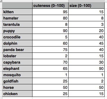
    "We'll begin by considering a small subset of English: words for animals. Our task is to be able to write computer programs to find similarities among these words and the creatures they designate. To do this, we might start by making a spreadsheet of some animals and their characteristics. For example:\n",
    "\n",
    "![Animal spreadsheet](http://static.decontextualize.com/snaps/animal-spreadsheet.png)\n",
    "\n",
    "This spreadsheet associates a handful of animals with two numbers: their cuteness and their size, both in a range from zero to one hundred. (The values themselves are simply based on my own judgment. Your taste in cuteness and evaluation of size may differ significantly from mine. As with all data, these data are simply a mirror reflection of the person who collected them.)\n",
    "\n",
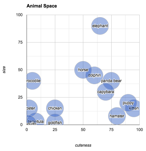
    "These values give us everything we need to make determinations about which animals are similar (at least, similar in the properties that we've included in the data). Try to answer the following question: Which animal is most similar to a capybara? You could go through the values one by one and do the math to make that evaluation, but visualizing the data as points in 2-dimensional space makes finding the answer very intuitive:\n",
    "\n",
    "![Animal space](http://static.decontextualize.com/snaps/animal-space.png)\n",
    "\n",
    "The plot shows us that the closest animal to the capybara is the panda bear (again, in terms of its subjective size and cuteness). One way of calculating how \"far apart\" two points are is to find their *Euclidean distance*. (This is simply the length of the line that connects the two points.) For points in two dimensions, Euclidean distance can be calculated with the following Python function:"
   ]
  },
  {
   "cell_type": "code",
   "execution_count": 325,
   "metadata": {},
   "outputs": [],
   "source": [
    "import math\n",
    "def distance2d(x1, y1, x2, y2):\n",
    "    return math.sqrt((x1 - x2)**2 + (y1 - y2)**2)"
   ]
  },
  {
   "cell_type": "markdown",
   "metadata": {},
   "source": [
    "(The `**` operator raises the value on its left to the power on its right.)\n",
    "\n",
    "So, the distance between \"capybara\" (70, 30) and \"panda\" (74, 40):"
   ]
  },
  {
   "cell_type": "code",
   "execution_count": 327,
   "metadata": {},
   "outputs": [
    {
     "data": {
      "text/plain": [
       "11.180339887498949"
      ]
     },
     "execution_count": 327,
     "metadata": {},
     "output_type": "execute_result"
    }
   ],
   "source": [
    "distance2d(70, 30, 75, 40) # panda and capybara"
   ]
  },
  {
   "cell_type": "markdown",
   "metadata": {},
   "source": [
    "... is less than the distance between \"tarantula\" and \"elephant\":"
   ]
  },
  {
   "cell_type": "code",
   "execution_count": 328,
   "metadata": {},
   "outputs": [
    {
     "data": {
      "text/plain": [
       "104.0096149401583"
      ]
     },
     "execution_count": 328,
     "metadata": {},
     "output_type": "execute_result"
    }
   ],
   "source": [
    "distance2d(8, 3, 65, 90) # tarantula and elephant"
   ]
  },
  {
   "cell_type": "markdown",
   "metadata": {},
   "source": [
    "Modeling animals in this way has a few other interesting properties. For example, you can pick an arbitrary point in \"animal space\" and then find the animal closest to that point. If you imagine an animal of size 25 and cuteness 30, you can easily look at the space to find the animal that most closely fits that description: the chicken.\n",
    "\n",
    "Reasoning visually, you can also answer questions like: what's halfway between a chicken and an elephant? Simply draw a line from \"elephant\" to \"chicken,\" mark off the midpoint and find the closest animal. (According to our chart, halfway between an elephant and a chicken is a horse.)\n",
    "\n",
    "You can also ask: what's the *difference* between a hamster and a tarantula? According to our plot, it's about seventy five units of cute (and a few units of size).\n",
    "\n",
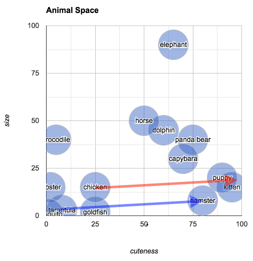
    "The relationship of \"difference\" is an interesting one, because it allows us to reason about *analogous* relationships. In the chart below, I've drawn an arrow from \"tarantula\" to \"hamster\" (in blue):\n",
    "\n",
    "![Animal analogy](http://static.decontextualize.com/snaps/animal-space-analogy.png)\n",
    "\n",
    "You can understand this arrow as being the *relationship* between a tarantula and a hamster, in terms of their size and cuteness (i.e., hamsters and tarantulas are about the same size, but hamsters are much cuter). In the same diagram, I've also transposed this same arrow (this time in red) so that its origin point is \"chicken.\" The arrow ends closest to \"kitten.\" What we've discovered is that the animal that is about the same size as a chicken but much cuter is... a kitten. To put it in terms of an analogy:\n",
    "\n",
    "    Tarantulas are to hamsters as chickens are to kittens.\n",
    "    \n",
    "A sequence of numbers used to identify a point is called a *vector*, and the kind of math we've been doing so far is called *linear algebra.* (Linear algebra is surprisingly useful across many domains: It's the same kind of math you might do to, e.g., simulate the velocity and acceleration of a sprite in a video game.)\n",
    "\n",
    "A set of vectors that are all part of the same data set is often called a *vector space*. The vector space of animals in this section has two *dimensions*, by which I mean that each vector in the space has two numbers associated with it (i.e., two columns in the spreadsheet). The fact that this space has two dimensions just happens to make it easy to *visualize* the space by drawing a 2D plot. But most vector spaces you'll work with will have more than two dimensions—sometimes many hundreds. In those cases, it's more difficult to visualize the \"space,\" but the math works pretty much the same."
   ]
  },
  {
   "cell_type": "markdown",
   "metadata": {},
   "source": [
    "## Language with vectors: colors\n",
    "\n",
    "So far, so good. We have a system in place—albeit highly subjective—for talking about animals and the words used to name them. I want to talk about another vector space that has to do with language: the vector space of colors.\n",
    "\n",
    "Colors are often represented in computers as vectors with three dimensions: red, green, and blue. Just as with the animals in the previous section, we can use these vectors to answer questions like: which colors are similar? What's the most likely color name for an arbitrarily chosen set of values for red, green and blue? Given the names of two colors, what's the name of those colors' \"average\"?\n",
    "\n",
    "We'll be working with this [color data](https://github.com/dariusk/corpora/blob/master/data/colors/xkcd.json) from the [xkcd color survey](https://blog.xkcd.com/2010/05/03/color-survey-results/). The data relates a color name to the RGB value associated with that color. [Here's a page that shows what the colors look like](https://xkcd.com/color/rgb/). Download the color data and put it in the same directory as this notebook.\n",
    "\n",
    "A few notes before we proceed:\n",
    "\n",
    "* The linear algebra functions implemented below (`addv`, `meanv`, etc.) are slow, potentially inaccurate, and shouldn't be used for \"real\" code—I wrote them so beginner programmers can understand how these kinds of functions work behind the scenes. Use [numpy](http://www.numpy.org/) for fast and accurate math in Python.\n",
    "* If you're interested in perceptually accurate color math in Python, consider using the [colormath library](http://python-colormath.readthedocs.io/en/latest/).\n",
    "\n",
    "Now, import the `json` library and load the color data:"
   ]
  },
  {
   "cell_type": "code",
   "execution_count": 329,
   "metadata": {
    "collapsed": true
   },
   "outputs": [],
   "source": [
    "import json"
   ]
  },
  {
   "cell_type": "code",
   "execution_count": 330,
   "metadata": {
    "collapsed": true
   },
   "outputs": [],
   "source": [
    "color_data = json.loads(open(\"xkcd.json\").read())"
   ]
  },
  {
   "cell_type": "markdown",
   "metadata": {},
   "source": [
    "The following function converts colors from hex format (`#1a2b3c`) to a tuple of integers:"
   ]
  },
  {
   "cell_type": "code",
   "execution_count": 331,
   "metadata": {
    "collapsed": true
   },
   "outputs": [],
   "source": [
    "def hex_to_int(s):\n",
    "    s = s.lstrip(\"#\")\n",
    "    return int(s[:2], 16), int(s[2:4], 16), int(s[4:6], 16)"
   ]
  },
  {
   "cell_type": "markdown",
   "metadata": {},
   "source": [
    "And the following cell creates a dictionary and populates it with mappings from color names to RGB vectors for each color in the data:"
   ]
  },
  {
   "cell_type": "code",
   "execution_count": 332,
   "metadata": {},
   "outputs": [],
   "source": [
    "colors = dict()\n",
    "for item in color_data['colors']:\n",
    "    colors[item[\"color\"]] = hex_to_int(item[\"hex\"])"
   ]
  },
  {
   "cell_type": "markdown",
   "metadata": {},
   "source": [
    "Testing it out:"
   ]
  },
  {
   "cell_type": "code",
   "execution_count": 338,
   "metadata": {},
   "outputs": [
    {
     "data": {
      "text/plain": [
       "(110, 117, 14)"
      ]
     },
     "execution_count": 338,
     "metadata": {},
     "output_type": "execute_result"
    }
   ],
   "source": [
    "colors['olive']"
   ]
  },
  {
   "cell_type": "code",
   "execution_count": 339,
   "metadata": {},
   "outputs": [
    {
     "data": {
      "text/plain": [
       "(229, 0, 0)"
      ]
     },
     "execution_count": 339,
     "metadata": {},
     "output_type": "execute_result"
    }
   ],
   "source": [
    "colors['red']"
   ]
  },
  {
   "cell_type": "code",
   "execution_count": 340,
   "metadata": {},
   "outputs": [
    {
     "data": {
      "text/plain": [
       "(0, 0, 0)"
      ]
     },
     "execution_count": 340,
     "metadata": {},
     "output_type": "execute_result"
    }
   ],
   "source": [
    "colors['black']"
   ]
  },
  {
   "cell_type": "markdown",
   "metadata": {},
   "source": [
    "### Vector math\n",
    "\n",
    "Before we keep going, we'll need some functions for performing basic vector \"arithmetic.\" These functions will work with vectors in spaces of any number of dimensions.\n",
    "\n",
    "The first function returns the Euclidean distance between two points:"
   ]
  },
  {
   "cell_type": "code",
   "execution_count": 341,
   "metadata": {
    "scrolled": true
   },
   "outputs": [
    {
     "data": {
      "text/plain": [
       "5.0990195135927845"
      ]
     },
     "execution_count": 341,
     "metadata": {},
     "output_type": "execute_result"
    }
   ],
   "source": [
    "import math\n",
    "def distance(coord1, coord2):\n",
    "    # note, this is VERY SLOW, don't use for actual code\n",
    "    return math.sqrt(sum([(i - j)**2 for i, j in zip(coord1, coord2)]))\n",
    "distance([10, 1], [5, 2])"
   ]
  },
  {
   "cell_type": "markdown",
   "metadata": {},
   "source": [
    "The `subtractv` function subtracts one vector from another:"
   ]
  },
  {
   "cell_type": "code",
   "execution_count": 342,
   "metadata": {},
   "outputs": [
    {
     "data": {
      "text/plain": [
       "[5, -1]"
      ]
     },
     "execution_count": 342,
     "metadata": {},
     "output_type": "execute_result"
    }
   ],
   "source": [
    "def subtractv(coord1, coord2):\n",
    "    return [c1 - c2 for c1, c2 in zip(coord1, coord2)]\n",
    "subtractv([10, 1], [5, 2])"
   ]
  },
  {
   "cell_type": "markdown",
   "metadata": {},
   "source": [
    "The `addv` vector adds two vectors together:"
   ]
  },
  {
   "cell_type": "code",
   "execution_count": 343,
   "metadata": {},
   "outputs": [
    {
     "data": {
      "text/plain": [
       "[15, 3]"
      ]
     },
     "execution_count": 343,
     "metadata": {},
     "output_type": "execute_result"
    }
   ],
   "source": [
    "def addv(coord1, coord2):\n",
    "    return [c1 + c2 for c1, c2 in zip(coord1, coord2)]\n",
    "addv([10, 1], [5, 2])"
   ]
  },
  {
   "cell_type": "markdown",
   "metadata": {},
   "source": [
    "And the `meanv` function takes a list of vectors and finds their mean or average:"
   ]
  },
  {
   "cell_type": "code",
   "execution_count": 344,
   "metadata": {},
   "outputs": [
    {
     "data": {
      "text/plain": [
       "[2.0, 2.0]"
      ]
     },
     "execution_count": 344,
     "metadata": {},
     "output_type": "execute_result"
    }
   ],
   "source": [
    "def meanv(coords):\n",
    "    # assumes every item in coords has same length as item 0\n",
    "    sumv = [0] * len(coords[0])\n",
    "    for item in coords:\n",
    "        for i in range(len(item)):\n",
    "            sumv[i] += item[i]\n",
    "    mean = [0] * len(sumv)\n",
    "    for i in range(len(sumv)):\n",
    "        mean[i] = float(sumv[i]) / len(coords)\n",
    "    return mean\n",
    "meanv([[0, 1], [2, 2], [4, 3]])"
   ]
  },
  {
   "cell_type": "markdown",
   "metadata": {},
   "source": [
    "Just as a test, the following cell shows that the distance from \"red\" to \"green\" is greater than the distance from \"red\" to \"pink\":"
   ]
  },
  {
   "cell_type": "code",
   "execution_count": 345,
   "metadata": {},
   "outputs": [
    {
     "data": {
      "text/plain": [
       "True"
      ]
     },
     "execution_count": 345,
     "metadata": {},
     "output_type": "execute_result"
    }
   ],
   "source": [
    "distance(colors['red'], colors['green']) > distance(colors['red'], colors['pink'])"
   ]
  },
  {
   "cell_type": "markdown",
   "metadata": {},
   "source": [
    "### Finding the closest item\n",
    "\n",
    "Just as we wanted to find the animal that most closely matched an arbitrary point in cuteness/size space, we'll want to find the closest color name to an arbitrary point in RGB space. The easiest way to find the closest item to an arbitrary vector is simply to find the distance between the target vector and each item in the space, in turn, then sort the list from closest to farthest. The `closest()` function below does just that. By default, it returns a list of the ten closest items to the given vector.\n",
    "\n",
    "> Note: Calculating \"closest neighbors\" like this is fine for the examples in this notebook, but unmanageably slow for vector spaces of any appreciable size. As your vector space grows, you'll want to move to a faster solution, like SciPy's [kdtree](https://docs.scipy.org/doc/scipy-0.14.0/reference/generated/scipy.spatial.KDTree.html) or [Annoy](https://pypi.python.org/pypi/annoy)."
   ]
  },
  {
   "cell_type": "code",
   "execution_count": 347,
   "metadata": {
    "collapsed": true
   },
   "outputs": [],
   "source": [
    "def closest(space, coord, n=10):\n",
    "    closest = []\n",
    "    for key in sorted(space.keys(),\n",
    "                        key=lambda x: distance(coord, space[x]))[:n]:\n",
    "        closest.append(key)\n",
    "    return closest"
   ]
  },
  {
   "cell_type": "markdown",
   "metadata": {},
   "source": [
    "Testing it out, we can find the ten colors closest to \"red\":"
   ]
  },
  {
   "cell_type": "code",
   "execution_count": 349,
   "metadata": {
    "scrolled": false
   },
   "outputs": [
    {
     "data": {
      "text/plain": [
       "[u'red',\n",
       " u'fire engine red',\n",
       " u'bright red',\n",
       " u'tomato red',\n",
       " u'cherry red',\n",
       " u'scarlet',\n",
       " u'vermillion',\n",
       " u'orangish red',\n",
       " u'cherry',\n",
       " u'lipstick red']"
      ]
     },
     "execution_count": 349,
     "metadata": {},
     "output_type": "execute_result"
    }
   ],
   "source": [
    "closest(colors, colors['red'])"
   ]
  },
  {
   "cell_type": "markdown",
   "metadata": {},
   "source": [
    "... or the ten colors closest to (150, 60, 150):"
   ]
  },
  {
   "cell_type": "code",
   "execution_count": 350,
   "metadata": {
    "scrolled": false
   },
   "outputs": [
    {
     "data": {
      "text/plain": [
       "[u'warm purple',\n",
       " u'medium purple',\n",
       " u'ugly purple',\n",
       " u'light eggplant',\n",
       " u'purpleish',\n",
       " u'purplish',\n",
       " u'purply',\n",
       " u'light plum',\n",
       " u'purple',\n",
       " u'muted purple']"
      ]
     },
     "execution_count": 350,
     "metadata": {},
     "output_type": "execute_result"
    }
   ],
   "source": [
    "closest(colors, [150, 60, 150])"
   ]
  },
  {
   "cell_type": "markdown",
   "metadata": {},
   "source": [
    "### Color magic\n",
    "\n",
    "The magical part of representing words as vectors is that the vector operations we defined earlier appear to operate on language the same way they operate on numbers. For example, if we find the word closest to the vector resulting from subtracting \"red\" from \"purple,\" we get a series of \"blue\" colors:"
   ]
  },
  {
   "cell_type": "code",
   "execution_count": 352,
   "metadata": {},
   "outputs": [
    {
     "data": {
      "text/plain": [
       "[u'cobalt blue',\n",
       " u'royal blue',\n",
       " u'darkish blue',\n",
       " u'true blue',\n",
       " u'royal',\n",
       " u'prussian blue',\n",
       " u'dark royal blue',\n",
       " u'deep blue',\n",
       " u'marine blue',\n",
       " u'deep sea blue']"
      ]
     },
     "execution_count": 352,
     "metadata": {},
     "output_type": "execute_result"
    }
   ],
   "source": [
    "closest(colors, subtractv(colors['purple'], colors['red']))"
   ]
  },
  {
   "cell_type": "markdown",
   "metadata": {},
   "source": [
    "This matches our intuition about RGB colors, which is that purple is a combination of red and blue. Take away the red, and blue is all you have left.\n",
    "\n",
    "You can do something similar with addition. What's blue plus green?"
   ]
  },
  {
   "cell_type": "code",
   "execution_count": 353,
   "metadata": {},
   "outputs": [
    {
     "data": {
      "text/plain": [
       "[u'bright turquoise',\n",
       " u'bright light blue',\n",
       " u'bright aqua',\n",
       " u'cyan',\n",
       " u'neon blue',\n",
       " u'aqua blue',\n",
       " u'bright cyan',\n",
       " u'bright sky blue',\n",
       " u'aqua',\n",
       " u'bright teal']"
      ]
     },
     "execution_count": 353,
     "metadata": {},
     "output_type": "execute_result"
    }
   ],
   "source": [
    "closest(colors, addv(colors['blue'], colors['green']))"
   ]
  },
  {
   "cell_type": "markdown",
   "metadata": {},
   "source": [
    "That's right, it's something like turquoise or cyan! What if we find the average of black and white? Predictably, we get gray:"
   ]
  },
  {
   "cell_type": "code",
   "execution_count": 355,
   "metadata": {},
   "outputs": [
    {
     "data": {
      "text/plain": [
       "[u'medium grey',\n",
       " u'purple grey',\n",
       " u'steel grey',\n",
       " u'battleship grey',\n",
       " u'grey purple',\n",
       " u'purplish grey',\n",
       " u'greyish purple',\n",
       " u'steel',\n",
       " u'warm grey',\n",
       " u'green grey']"
      ]
     },
     "execution_count": 355,
     "metadata": {},
     "output_type": "execute_result"
    }
   ],
   "source": [
    "# the average of black and white: medium grey\n",
    "closest(colors, meanv([colors['black'], colors['white']]))"
   ]
  },
  {
   "cell_type": "markdown",
   "metadata": {},
   "source": [
    "Just as with the tarantula/hamster example from the previous section, we can use color vectors to reason about relationships between colors. In the cell below, finding the difference between \"pink\" and \"red\" then adding it to \"blue\" seems to give us a list of colors that are to blue what pink is to red (i.e., a slightly lighter, less saturated shade):"
   ]
  },
  {
   "cell_type": "code",
   "execution_count": 354,
   "metadata": {},
   "outputs": [
    {
     "data": {
      "text/plain": [
       "[u'neon blue',\n",
       " u'bright sky blue',\n",
       " u'bright light blue',\n",
       " u'cyan',\n",
       " u'bright cyan',\n",
       " u'bright turquoise',\n",
       " u'clear blue',\n",
       " u'azure',\n",
       " u'dodger blue',\n",
       " u'lightish blue']"
      ]
     },
     "execution_count": 354,
     "metadata": {},
     "output_type": "execute_result"
    }
   ],
   "source": [
    "# an analogy: pink is to red as X is to blue\n",
    "pink_to_red = subtractv(colors['pink'], colors['red'])\n",
    "closest(colors, addv(pink_to_red, colors['blue']))"
   ]
  },
  {
   "cell_type": "markdown",
   "metadata": {},
   "source": [
    "Another example of color analogies: Navy is to blue as true green/dark grass green is to green:"
   ]
  },
  {
   "cell_type": "code",
   "execution_count": 358,
   "metadata": {},
   "outputs": [
    {
     "data": {
      "text/plain": [
       "[u'true green',\n",
       " u'dark grass green',\n",
       " u'grassy green',\n",
       " u'racing green',\n",
       " u'forest',\n",
       " u'bottle green',\n",
       " u'dark olive green',\n",
       " u'darkgreen',\n",
       " u'forrest green',\n",
       " u'grass green']"
      ]
     },
     "execution_count": 358,
     "metadata": {},
     "output_type": "execute_result"
    }
   ],
   "source": [
    "# another example: \n",
    "navy_to_blue = subtractv(colors['navy'], colors['blue'])\n",
    "closest(colors, addv(navy_to_blue, colors['green']))"
   ]
  },
  {
   "cell_type": "markdown",
   "metadata": {},
   "source": [
    "The examples above are fairly simple from a mathematical perspective but nevertheless *feel* magical: they're demonstrating that it's possible to use math to reason about how people use language."
   ]
  },
  {
   "cell_type": "markdown",
   "metadata": {},
   "source": [
    "### Interlude: A Love Poem That Loses Its Way"
   ]
  },
  {
   "cell_type": "code",
   "execution_count": 378,
   "metadata": {},
   "outputs": [
    {
     "name": "stdout",
     "output_type": "stream",
     "text": [
      "Roses are red, violets are blue\n",
      "Roses are tomato red, violets are electric blue\n",
      "Roses are deep orange, violets are deep sky blue\n",
      "Roses are burnt orange, violets are bright blue\n",
      "Roses are brick orange, violets are cerulean\n",
      "Roses are dark orange, violets are turquoise blue\n",
      "Roses are orange brown, violets are teal blue\n",
      "Roses are brown orange, violets are peacock blue\n",
      "Roses are dirty orange, violets are deep aqua\n",
      "Roses are pumpkin, violets are dark cyan\n",
      "Roses are orange, violets are ocean\n",
      "Roses are deep orange, violets are greenish blue\n",
      "Roses are rusty orange, violets are dark cyan\n",
      "Roses are burnt orange, violets are sea blue\n"
     ]
    }
   ],
   "source": [
    "import random\n",
    "red = colors['red']\n",
    "blue = colors['blue']\n",
    "for i in range(14):\n",
    "    rednames = closest(colors, red)\n",
    "    bluenames = closest(colors, blue)\n",
    "    print \"Roses are \" + rednames[0] + \", violets are \" + bluenames[0]\n",
    "    red = colors[random.choice(rednames[1:])]\n",
    "    blue = colors[random.choice(bluenames[1:])]"
   ]
  },
  {
   "cell_type": "markdown",
   "metadata": {},
   "source": [
    "### Doing bad digital humanities with color vectors\n",
    "\n",
    "With the tools above in hand, we can start using our vectorized knowledge of language toward academic ends. In the following example, I'm going to calculate the average color of Bram Stoker's *Dracula*.\n",
    "\n",
    "(Before you proceed, make sure to [download the text file from Project Gutenberg](http://www.gutenberg.org/cache/epub/345/pg345.txt) and place it in the same directory as this notebook.)\n",
    "\n",
    "First, we'll load [spaCy](https://spacy.io/):"
   ]
  },
  {
   "cell_type": "code",
   "execution_count": 359,
   "metadata": {
    "collapsed": true
   },
   "outputs": [],
   "source": [
    "import spacy\n",
    "nlp = spacy.load('en')"
   ]
  },
  {
   "cell_type": "markdown",
   "metadata": {},
   "source": [
    "To calculate the average color, we'll follow these steps:\n",
    "\n",
    "1. Parse the text into words\n",
    "2. Check every word to see if it names a color in our vector space. If it does, add it to a list of vectors.\n",
    "3. Find the average of that list of vectors.\n",
    "4. Find the color(s) closest to that average vector.\n",
    "\n",
    "The following cell performs steps 1-3:"
   ]
  },
  {
   "cell_type": "code",
   "execution_count": 370,
   "metadata": {},
   "outputs": [
    {
     "name": "stdout",
     "output_type": "stream",
     "text": [
      "[147.44839067702551, 113.65371809100999, 100.13540510543841]\n"
     ]
    }
   ],
   "source": [
    "doc = nlp(open(\"pg345.txt\").read().decode('utf8'))\n",
    "# use word.lower_ to normalize case\n",
    "drac_colors = [colors[word.lower_] for word in doc if word.lower_ in colors]\n",
    "avg_color = meanv(drac_colors)\n",
    "print avg_color"
   ]
  },
  {
   "cell_type": "markdown",
   "metadata": {},
   "source": [
    "Now, we'll pass the averaged color vector to the `closest()` function, yielding... well, it's just a brown mush, which is kinda what you'd expect from adding a bunch of colors together willy-nilly."
   ]
  },
  {
   "cell_type": "code",
   "execution_count": 371,
   "metadata": {},
   "outputs": [
    {
     "data": {
      "text/plain": [
       "[u'reddish grey',\n",
       " u'brownish grey',\n",
       " u'brownish',\n",
       " u'brown grey',\n",
       " u'mocha',\n",
       " u'grey brown',\n",
       " u'puce',\n",
       " u'dull brown',\n",
       " u'pinkish brown',\n",
       " u'dark taupe']"
      ]
     },
     "execution_count": 371,
     "metadata": {},
     "output_type": "execute_result"
    }
   ],
   "source": [
    "closest(colors, avg_color)"
   ]
  },
  {
   "cell_type": "markdown",
   "metadata": {},
   "source": [
    "On the other hand, here's what we get when we average the colors of Charlotte Perkins Gilman's classic *The Yellow Wallpaper*. ([Download from here](http://www.gutenberg.org/cache/epub/1952/pg1952.txt) and save in the same directory as this notebook if you want to follow along.) The result definitely reflects the content of the story, so maybe we're on to something here."
   ]
  },
  {
   "cell_type": "code",
   "execution_count": 369,
   "metadata": {},
   "outputs": [
    {
     "data": {
      "text/plain": [
       "[u'sickly yellow',\n",
       " u'piss yellow',\n",
       " u'puke yellow',\n",
       " u'vomit yellow',\n",
       " u'dirty yellow',\n",
       " u'mustard yellow',\n",
       " u'dark yellow',\n",
       " u'olive yellow',\n",
       " u'macaroni and cheese',\n",
       " u'pea']"
      ]
     },
     "execution_count": 369,
     "metadata": {},
     "output_type": "execute_result"
    }
   ],
   "source": [
    "doc = nlp(open(\"pg1952.txt\").read().decode('utf8'))\n",
    "wallpaper_colors = [colors[word.lower_] for word in doc if word.lower_ in colors]\n",
    "avg_color = meanv(wallpaper_colors)\n",
    "closest(colors, avg_color)"
   ]
  },
  {
   "cell_type": "markdown",
   "metadata": {},
   "source": [
    "Exercise for the reader: Use the vector arithmetic functions to rewrite a text, making it...\n",
    "\n",
    "* more blue (i.e., add `colors['blue']` to each occurrence of a color word); or\n",
    "* more light (i.e., add `colors['white']` to each occurrence of a color word); or\n",
    "* darker (i.e., attenuate each color. You might need to write a vector multiplication function to do this one right.)"
   ]
  },
  {
   "cell_type": "markdown",
   "metadata": {},
   "source": [
    "## Distributional semantics\n",
    "\n",
    "In the previous section, the examples are interesting because of a simple fact: colors that we think of as similar are \"closer\" to each other in RGB vector space. In our color vector space, or in our animal cuteness/size space, you can think of the words identified by vectors close to each other as being *synonyms*, in a sense: they sort of \"mean\" the same thing. They're also, for many purposes, *functionally identical*. Think of this in terms of writing, say, a search engine. If someone searches for \"mauve trousers,\" then it's probably also okay to show them results for, say,"
   ]
  },
  {
   "cell_type": "code",
   "execution_count": 380,
   "metadata": {},
   "outputs": [
    {
     "name": "stdout",
     "output_type": "stream",
     "text": [
      "mauve trousers\n",
      "dusty rose trousers\n",
      "dusky rose trousers\n",
      "brownish pink trousers\n",
      "old pink trousers\n",
      "reddish grey trousers\n",
      "dirty pink trousers\n",
      "old rose trousers\n",
      "light plum trousers\n",
      "ugly pink trousers\n"
     ]
    }
   ],
   "source": [
    "for cname in closest(colors, colors['mauve']):\n",
    "    print cname + \" trousers\""
   ]
  },
  {
   "cell_type": "markdown",
   "metadata": {},
   "source": [
    "That's all well and good for color words, which intuitively seem to exist in a multidimensional continuum of perception, and for our animal space, where we've written out the vectors ahead of time. But what about... arbitrary words? Is it possible to create a vector space for all English words that has this same \"closer in space is closer in meaning\" property?\n",
    "\n",
    "To answer that, we have to back up a bit and ask the question: what does *meaning* mean? No one really knows, but one theory popular among computational linguists, computer scientists and other people who make search engines is the [Distributional Hypothesis](https://en.wikipedia.org/wiki/Distributional_semantics), which states that:\n",
    "\n",
    "    Linguistic items with similar distributions have similar meanings.\n",
    "    \n",
    "What's meant by \"similar distributions\" is *similar contexts*. Take for example the following sentences:\n",
    "\n",
    "    It was really cold yesterday.\n",
    "    It will be really warm today, though.\n",
    "    It'll be really hot tomorrow!\n",
    "    Will it be really cool Tuesday?\n",
    "    \n",
    "According to the Distributional Hypothesis, the words `cold`, `warm`, `hot` and `cool` must be related in some way (i.e., be close in meaning) because they occur in a similar context, i.e., between the word \"really\" and a word indicating a particular day. (Likewise, the words `yesterday`, `today`, `tomorrow` and `Tuesday` must be related, since they occur in the context of a word indicating a temperature.)\n",
    "\n",
    "In other words, according to the Distributional Hypothesis, a word's meaning is just a big list of all the contexts it occurs in. Two words are closer in meaning if they share contexts."
   ]
  },
  {
   "attachments": {},
   "cell_type": "markdown",
   "metadata": {},
   "source": [
    "## Word vectors by counting contexts\n",
    "\n",
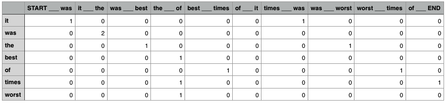
    "So how do we turn this insight from the Distributional Hypothesis into a system for creating general-purpose vectors that capture the meaning of words? Maybe you can see where I'm going with this. What if we made a *really big* spreadsheet that had one column for every context for every word in a given source text. Let's use a small source text to begin with, such as this excerpt from Dickens:\n",
    "\n",
    "    It was the best of times, it was the worst of times.\n",
    "\n",
    "Such a spreadsheet might look something like this:\n",
    "\n",
    "![dickens contexts](http://static.decontextualize.com/snaps/best-of-times.png)\n",
    "\n",
    "The spreadsheet has one column for every possible context, and one row for every word. The values in each cell correspond with how many times the word occurs in the given context. The numbers in the columns constitute that word's vector, i.e., the vector for the word `of` is\n",
    "\n",
    "    [0, 0, 0, 0, 1, 0, 0, 0, 1, 0]\n",
    "    \n",
    "Because there are ten possible contexts, this is a ten dimensional space! It might be strange to think of it, but you can do vector arithmetic on vectors with ten dimensions just as easily as you can on vectors with two or three dimensions, and you could use the same distance formula that we defined earlier to get useful information about which vectors in this space are similar to each other. In particular, the vectors for `best` and `worst` are actually the same (a distance of zero), since they occur only in the same context (`the ___ of`):\n",
    "\n",
    "    [0, 0, 0, 1, 0, 0, 0, 0, 0, 0]\n",
    "    \n",
    "Of course, the conventional way of thinking about \"best\" and \"worst\" is that they're *antonyms*, not *synonyms*. But they're also clearly two words of the same kind, with related meanings (through opposition), a fact that is captured by this distributional model.\n",
    "\n",
    "### Contexts and dimensionality\n",
    "\n",
    "Of course, in a corpus of any reasonable size, there will be many thousands if not many millions of possible contexts. It's difficult enough working with a vector space of ten dimensions, let alone a vector space of a million dimensions! It turns out, though, that many of the dimensions end up being superfluous and can either be eliminated or combined with other dimensions without significantly affecting the predictive power of the resulting vectors. The process of getting rid of superfluous dimensions in a vector space is called [dimensionality reduction](https://en.wikipedia.org/wiki/Dimensionality_reduction), and most implementations of count-based word vectors make use of dimensionality reduction so that the resulting vector space has a reasonable number of dimensions (say, 100—300, depending on the corpus and application).\n",
    "\n",
    "The question of how to identify a \"context\" is itself very difficult to answer. In the toy example above, we've said that a \"context\" is just the word that precedes and the word that follows. Depending on your implementation of this procedure, though, you might want a context with a bigger \"window\" (e.g., two words before and after), or a non-contiguous window (skip a word before and after the given word). You might exclude certain \"function\" words like \"the\" and \"of\" when determining a word's context, or you might [lemmatize](https://en.wikipedia.org/wiki/Lemmatisation) the words before you begin your analysis, so two occurrences with different \"forms\" of the same word count as the same context. These are all questions open to research and debate, and different implementations of procedures for creating count-based word vectors make different decisions on this issue.\n",
    "\n",
    "### GloVe vectors\n",
    "\n",
    "But you don't have to create your own word vectors from scratch! Many researchers have made downloadable databases of pre-trained vectors. One such project is Stanford's [Global Vectors for Word Representation (GloVe)](https://nlp.stanford.edu/projects/glove/). These 300-dimensional vectors are included with spaCy, and they're the vectors we'll be using for the rest of this tutorial."
   ]
  },
  {
   "cell_type": "markdown",
   "metadata": {},
   "source": [
    "## Word vectors in spaCy\n",
    "\n",
    "Okay, let's have some fun with real word vectors. We're going to use the GloVe vectors that come with spaCy to creatively analyze and manipulate the text of Bram Stoker's *Dracula*. First, make sure you've got `spacy` imported:"
   ]
  },
  {
   "cell_type": "code",
   "execution_count": 381,
   "metadata": {
    "collapsed": true
   },
   "outputs": [],
   "source": [
    "from __future__ import unicode_literals\n",
    "import spacy"
   ]
  },
  {
   "cell_type": "markdown",
   "metadata": {},
   "source": [
    "The following cell loads the language model and parses the input text:"
   ]
  },
  {
   "cell_type": "code",
   "execution_count": 382,
   "metadata": {},
   "outputs": [],
   "source": [
    "nlp = spacy.load('en')\n",
    "doc = nlp(open(\"pg345.txt\").read().decode('utf8'))"
   ]
  },
  {
   "cell_type": "markdown",
   "metadata": {},
   "source": [
    "And the cell below creates a list of unique words (or tokens) in the text, as a list of strings."
   ]
  },
  {
   "cell_type": "code",
   "execution_count": 383,
   "metadata": {
    "collapsed": true
   },
   "outputs": [],
   "source": [
    "# all of the words in the text file\n",
    "tokens = list(set([w.text for w in doc if w.is_alpha]))"
   ]
  },
  {
   "cell_type": "markdown",
   "metadata": {},
   "source": [
    "You can see the vector of any word in spaCy's vocabulary using the `vocab` attribute, like so:"
   ]
  },
  {
   "cell_type": "code",
   "execution_count": 385,
   "metadata": {
    "scrolled": true
   },
   "outputs": [
    {
     "data": {
      "text/plain": [
       "array([ -5.52519977e-01,   1.88940004e-01,   6.87370002e-01,\n",
       "        -1.97889999e-01,   7.05749989e-02,   1.00750005e+00,\n",
       "         5.17890006e-02,  -1.56029999e-01,   3.19409996e-01,\n",
       "         1.17019999e+00,  -4.72479999e-01,   4.28669989e-01,\n",
       "        -4.20249999e-01,   2.48030007e-01,   6.81940019e-01,\n",
       "        -6.74880028e-01,   9.24009979e-02,   1.30890000e+00,\n",
       "        -3.62779982e-02,   2.00979993e-01,   7.60049999e-01,\n",
       "        -6.67179972e-02,  -7.77940005e-02,   2.38440007e-01,\n",
       "        -2.43509993e-01,  -5.41639984e-01,  -3.35399985e-01,\n",
       "         2.98049986e-01,   3.52690011e-01,  -8.05939972e-01,\n",
       "        -4.36109990e-01,   6.15350008e-01,   3.42119992e-01,\n",
       "        -3.36030006e-01,   3.32819998e-01,   3.80650014e-01,\n",
       "         5.74270003e-02,   9.99180004e-02,   1.25249997e-01,\n",
       "         1.10389996e+00,   3.66780013e-02,   3.04899991e-01,\n",
       "        -1.49419993e-01,   3.29120010e-01,   2.32999995e-01,\n",
       "         4.33950007e-01,   1.56660005e-01,   2.27779999e-01,\n",
       "        -2.58300006e-02,   2.43340001e-01,  -5.81360012e-02,\n",
       "        -1.34859994e-01,   2.45210007e-01,  -3.34589988e-01,\n",
       "         4.28389996e-01,  -4.81810004e-01,   1.34029999e-01,\n",
       "         2.60490000e-01,   8.99330005e-02,  -9.37699974e-02,\n",
       "         3.76720011e-01,  -2.95579992e-02,   4.38410014e-01,\n",
       "         6.12119973e-01,  -2.57200003e-01,  -7.85059988e-01,\n",
       "         2.38800004e-01,   1.33990005e-01,  -7.93149993e-02,\n",
       "         7.05820024e-01,   3.99679989e-01,   6.77789986e-01,\n",
       "        -2.04739999e-03,   1.97850000e-02,  -4.20590013e-01,\n",
       "        -5.38580000e-01,  -5.21549992e-02,   1.72519997e-01,\n",
       "         2.75469989e-01,  -4.44819987e-01,   2.35949993e-01,\n",
       "        -2.34449998e-01,   3.01030010e-01,  -5.50960004e-01,\n",
       "        -3.11590005e-02,  -3.44330013e-01,   1.23860002e+00,\n",
       "         1.03170002e+00,  -2.27280006e-01,  -9.52070020e-03,\n",
       "        -2.54319996e-01,  -2.97919989e-01,   2.59339988e-01,\n",
       "        -1.04209997e-01,  -3.38759989e-01,   4.24699992e-01,\n",
       "         5.83350018e-04,   1.30930007e-01,   2.87860006e-01,\n",
       "         2.34740004e-01,   2.59050000e-02,  -6.43589973e-01,\n",
       "         6.13300018e-02,   6.38419986e-01,   1.47049993e-01,\n",
       "        -6.15939975e-01,   2.50970006e-01,  -4.48720008e-01,\n",
       "         8.68250012e-01,   9.95550007e-02,  -4.47340012e-02,\n",
       "        -7.42389977e-01,  -5.91470003e-01,  -5.49290001e-01,\n",
       "         3.81080002e-01,   5.51769994e-02,  -1.04869999e-01,\n",
       "        -1.28380001e-01,   6.05210010e-03,   2.87429988e-01,\n",
       "         2.15920001e-01,   7.28709996e-02,  -3.16439986e-01,\n",
       "        -4.33209985e-01,   1.86820000e-01,   6.72739968e-02,\n",
       "         2.81150013e-01,  -4.62220013e-02,  -9.68030021e-02,\n",
       "         5.60909986e-01,  -6.77619994e-01,  -1.66449994e-01,\n",
       "         1.55530006e-01,   5.23010015e-01,  -3.00579995e-01,\n",
       "        -3.72909993e-01,   8.78949985e-02,  -1.79629996e-01,\n",
       "        -4.41929996e-01,  -4.46069986e-01,  -2.41219997e+00,\n",
       "         3.37379992e-01,   6.24159992e-01,   4.27870005e-01,\n",
       "        -2.53859997e-01,  -6.16829991e-01,  -7.00969994e-01,\n",
       "         4.93030012e-01,   3.69159997e-01,  -9.74989980e-02,\n",
       "         6.14109993e-01,  -4.75719990e-03,   4.39159989e-01,\n",
       "        -2.15509996e-01,  -5.67449987e-01,  -4.02779996e-01,\n",
       "         2.94589996e-01,  -3.08499992e-01,   1.01030000e-01,\n",
       "         7.97410011e-02,  -6.38109982e-01,   2.47810006e-01,\n",
       "        -4.45459992e-01,   1.08280003e-01,  -2.36240000e-01,\n",
       "        -5.08379996e-01,  -1.70010000e-01,  -7.87349999e-01,\n",
       "         3.40730011e-01,  -3.18300009e-01,   4.52859998e-01,\n",
       "        -9.51180011e-02,   2.07719997e-01,  -8.01829994e-02,\n",
       "        -3.79819989e-01,  -4.99489993e-01,   4.07590009e-02,\n",
       "        -3.77240002e-01,  -8.97049978e-02,  -6.81869984e-01,\n",
       "         2.21059993e-01,  -3.99309993e-01,   3.23289990e-01,\n",
       "        -3.61799985e-01,  -7.20929980e-01,  -6.34039998e-01,\n",
       "         4.31250006e-01,  -4.97429997e-01,  -1.73950002e-01,\n",
       "        -3.87789994e-01,  -3.25560004e-01,   1.44229993e-01,\n",
       "        -8.34010020e-02,  -2.29939997e-01,   2.77929991e-01,\n",
       "         4.91120011e-01,   6.45110011e-01,  -7.89450034e-02,\n",
       "         1.11709997e-01,   3.72640014e-01,   1.30700007e-01,\n",
       "        -6.16069995e-02,  -4.35009986e-01,   2.89990008e-02,\n",
       "         5.62240005e-01,   5.80120012e-02,   4.70779985e-02,\n",
       "         4.27700013e-01,   7.32450008e-01,  -2.11500004e-02,\n",
       "         1.19879998e-01,   7.88230002e-02,  -1.91060007e-01,\n",
       "         3.52779999e-02,  -3.11019987e-01,   1.32090002e-01,\n",
       "        -2.86060005e-01,  -1.56489998e-01,  -6.43390000e-01,\n",
       "         4.45989996e-01,  -3.09119999e-01,   4.45199996e-01,\n",
       "        -3.67740005e-01,   2.73270011e-01,   6.78330004e-01,\n",
       "        -8.38299990e-02,  -4.51200008e-01,   1.07539997e-01,\n",
       "        -4.59080011e-01,   1.50950000e-01,  -4.58559990e-01,\n",
       "         3.44650000e-01,   7.80130029e-02,  -2.83190012e-01,\n",
       "        -2.81489994e-02,   2.44039997e-01,  -7.13450015e-01,\n",
       "         5.28340004e-02,  -2.80849993e-01,   2.53439993e-02,\n",
       "         4.29789983e-02,   1.56629995e-01,  -7.46469975e-01,\n",
       "        -1.13010001e+00,   4.41350013e-01,   3.14440012e-01,\n",
       "        -1.00180000e-01,  -5.35260022e-01,  -9.06009972e-01,\n",
       "        -6.49540007e-01,   4.26639989e-02,  -7.99269974e-02,\n",
       "         3.29050004e-01,  -3.07969987e-01,  -1.91900004e-02,\n",
       "         4.27650005e-01,   3.14599991e-01,   2.90509999e-01,\n",
       "        -2.73860008e-01,   6.84830010e-01,   1.93949994e-02,\n",
       "        -3.28839988e-01,  -4.82389987e-01,  -1.57470003e-01,\n",
       "        -1.60359994e-01,   4.91640002e-01,  -7.03520000e-01,\n",
       "        -3.55910003e-01,  -7.48870015e-01,  -5.28270006e-01,\n",
       "         4.49829996e-02,   5.92469983e-02,   4.62240010e-01,\n",
       "         8.96970034e-02,  -7.56179988e-01,   6.36820018e-01,\n",
       "         9.06800032e-02,   6.88299984e-02,   1.82960004e-01,\n",
       "         1.07539997e-01,   6.78110003e-01,  -1.47159994e-01,\n",
       "         1.70289993e-01,  -5.26300013e-01,   1.92680001e-01,\n",
       "         9.31299984e-01,   8.03629994e-01,   6.13240004e-01,\n",
       "        -3.04939985e-01,   2.02360004e-01,   5.85200012e-01,\n",
       "         2.64840007e-01,  -4.58629996e-01,   2.10350007e-03,\n",
       "        -5.69899976e-01,  -4.90920007e-01,   4.25110012e-01,\n",
       "        -1.09539998e+00,   1.71240002e-01,   2.24950001e-01], dtype=float32)"
      ]
     },
     "execution_count": 385,
     "metadata": {},
     "output_type": "execute_result"
    }
   ],
   "source": [
    "nlp.vocab['cheese'].vector"
   ]
  },
  {
   "cell_type": "markdown",
   "metadata": {},
   "source": [
    "For the sake of convenience, the following function gets the vector of a given string from spaCy's vocabulary:"
   ]
  },
  {
   "cell_type": "code",
   "execution_count": 384,
   "metadata": {
    "collapsed": true
   },
   "outputs": [],
   "source": [
    "def vec(s):\n",
    "    return nlp.vocab[s].vector"
   ]
  },
  {
   "cell_type": "markdown",
   "metadata": {},
   "source": [
    "### Cosine similarity and finding closest neighbors\n",
    "\n",
    "The cell below defines a function `cosine()`, which returns the [cosine similarity](https://en.wikipedia.org/wiki/Cosine_similarity) of two vectors. Cosine similarity is another way of determining how similar two vectors are, which is more suited to high-dimensional spaces. [See the Encyclopedia of Distances for more information and even more ways of determining vector similarity.](http://www.uco.es/users/ma1fegan/Comunes/asignaturas/vision/Encyclopedia-of-distances-2009.pdf)\n",
    "\n",
    "(You'll need to install `numpy` to get this to work. If you haven't already: `pip install numpy`. Use `sudo` if you need to and make sure you've upgraded to the most recent version of `pip` with `sudo pip install --upgrade pip`.)"
   ]
  },
  {
   "cell_type": "code",
   "execution_count": 387,
   "metadata": {
    "collapsed": true
   },
   "outputs": [],
   "source": [
    "import numpy as np\n",
    "from numpy import dot\n",
    "from numpy.linalg import norm\n",
    "\n",
    "# cosine similarity\n",
    "def cosine(v1, v2):\n",
    "    if norm(v1) > 0 and norm(v2) > 0:\n",
    "        return dot(v1, v2) / (norm(v1) * norm(v2))\n",
    "    else:\n",
    "        return 0.0"
   ]
  },
  {
   "cell_type": "markdown",
   "metadata": {},
   "source": [
    "The following cell shows that the cosine similarity between `dog` and `puppy` is larger than the similarity between `trousers` and `octopus`, thereby demonstrating that the vectors are working how we expect them to:"
   ]
  },
  {
   "cell_type": "code",
   "execution_count": 389,
   "metadata": {
    "scrolled": false
   },
   "outputs": [
    {
     "data": {
      "text/plain": [
       "True"
      ]
     },
     "execution_count": 389,
     "metadata": {},
     "output_type": "execute_result"
    }
   ],
   "source": [
    "cosine(vec('dog'), vec('puppy')) > cosine(vec('trousers'), vec('octopus'))"
   ]
  },
  {
   "cell_type": "markdown",
   "metadata": {},
   "source": [
    "The following cell defines a function that iterates through a list of tokens and returns the token whose vector is most similar to a given vector."
   ]
  },
  {
   "cell_type": "code",
   "execution_count": 390,
   "metadata": {
    "collapsed": true
   },
   "outputs": [],
   "source": [
    "def spacy_closest(token_list, vec_to_check, n=10):\n",
    "    return sorted(token_list,\n",
    "                  key=lambda x: cosine(vec_to_check, vec(x)),\n",
    "                  reverse=True)[:n]"
   ]
  },
  {
   "cell_type": "markdown",
   "metadata": {},
   "source": [
    "Using this function, we can get a list of synonyms, or words closest in meaning (or distribution, depending on how you look at it), to any arbitrary word in spaCy's vocabulary. In the following example, we're finding the words in *Dracula* closest to \"basketball\":"
   ]
  },
  {
   "cell_type": "code",
   "execution_count": 391,
   "metadata": {
    "scrolled": true
   },
   "outputs": [
    {
     "data": {
      "text/plain": [
       "[u'tennis',\n",
       " u'coach',\n",
       " u'game',\n",
       " u'teams',\n",
       " u'Junior',\n",
       " u'junior',\n",
       " u'Team',\n",
       " u'school',\n",
       " u'boys',\n",
       " u'leagues']"
      ]
     },
     "execution_count": 391,
     "metadata": {},
     "output_type": "execute_result"
    }
   ],
   "source": [
    "# what's the closest equivalent of basketball?\n",
    "spacy_closest(tokens, vec(\"basketball\"))"
   ]
  },
  {
   "cell_type": "markdown",
   "metadata": {},
   "source": [
    "### Fun with spaCy, Dracula, and vector arithmetic\n",
    "\n",
    "Now we can start doing vector arithmetic and finding the closest words to the resulting vectors. For example, what word is closest to the halfway point between day and night?"
   ]
  },
  {
   "cell_type": "code",
   "execution_count": 393,
   "metadata": {},
   "outputs": [
    {
     "data": {
      "text/plain": [
       "[u'night',\n",
       " u'day',\n",
       " u'Day',\n",
       " u'evening',\n",
       " u'Evening',\n",
       " u'Morning',\n",
       " u'morning',\n",
       " u'afternoon',\n",
       " u'Nights',\n",
       " u'nights']"
      ]
     },
     "execution_count": 393,
     "metadata": {},
     "output_type": "execute_result"
    }
   ],
   "source": [
    "# halfway between day and night\n",
    "spacy_closest(tokens, meanv([vec(\"day\"), vec(\"night\")]))"
   ]
  },
  {
   "cell_type": "markdown",
   "metadata": {},
   "source": [
    "Variations of `night` and `day` are still closest, but after that we get words like `evening` and `morning`, which are indeed halfway between day and night!"
   ]
  },
  {
   "cell_type": "markdown",
   "metadata": {},
   "source": [
    "Here are the closest words in _Dracula_ to \"wine\":"
   ]
  },
  {
   "cell_type": "code",
   "execution_count": 395,
   "metadata": {},
   "outputs": [
    {
     "data": {
      "text/plain": [
       "[u'wine',\n",
       " u'beer',\n",
       " u'bottle',\n",
       " u'Drink',\n",
       " u'drink',\n",
       " u'fruit',\n",
       " u'bottles',\n",
       " u'taste',\n",
       " u'coffee',\n",
       " u'tasted']"
      ]
     },
     "execution_count": 395,
     "metadata": {},
     "output_type": "execute_result"
    }
   ],
   "source": [
    "spacy_closest(tokens, vec(\"wine\"))"
   ]
  },
  {
   "cell_type": "markdown",
   "metadata": {},
   "source": [
    "If you subtract \"alcohol\" from \"wine\" and find the closest words to the resulting vector, you're left with simply a lovely dinner:"
   ]
  },
  {
   "cell_type": "code",
   "execution_count": 397,
   "metadata": {},
   "outputs": [
    {
     "data": {
      "text/plain": [
       "[u'wine',\n",
       " u'Dinner',\n",
       " u'dinner',\n",
       " u'lovely',\n",
       " u'delicious',\n",
       " u'salad',\n",
       " u'treasure',\n",
       " u'wonderful',\n",
       " u'Wonderful',\n",
       " u'cheese']"
      ]
     },
     "execution_count": 397,
     "metadata": {},
     "output_type": "execute_result"
    }
   ],
   "source": [
    "spacy_closest(tokens, subtractv(vec(\"wine\"), vec(\"alcohol\")))"
   ]
  },
  {
   "cell_type": "markdown",
   "metadata": {},
   "source": [
    "The closest words to \"water\":"
   ]
  },
  {
   "cell_type": "code",
   "execution_count": 398,
   "metadata": {},
   "outputs": [
    {
     "data": {
      "text/plain": [
       "[u'water',\n",
       " u'waters',\n",
       " u'salt',\n",
       " u'Salt',\n",
       " u'dry',\n",
       " u'liquid',\n",
       " u'ocean',\n",
       " u'boiling',\n",
       " u'heat',\n",
       " u'sand']"
      ]
     },
     "execution_count": 398,
     "metadata": {},
     "output_type": "execute_result"
    }
   ],
   "source": [
    "spacy_closest(tokens, vec(\"water\"))"
   ]
  },
  {
   "cell_type": "markdown",
   "metadata": {},
   "source": [
    "But if you add \"frozen\" to \"water,\" you get \"ice\":"
   ]
  },
  {
   "cell_type": "code",
   "execution_count": 400,
   "metadata": {},
   "outputs": [
    {
     "data": {
      "text/plain": [
       "[u'water',\n",
       " u'cold',\n",
       " u'ice',\n",
       " u'salt',\n",
       " u'Salt',\n",
       " u'dry',\n",
       " u'fresh',\n",
       " u'liquid',\n",
       " u'boiling',\n",
       " u'milk']"
      ]
     },
     "execution_count": 400,
     "metadata": {},
     "output_type": "execute_result"
    }
   ],
   "source": [
    "spacy_closest(tokens, addv(vec(\"water\"), vec(\"frozen\")))"
   ]
  },
  {
   "cell_type": "markdown",
   "metadata": {},
   "source": [
    "You can even do analogies! For example, the words most similar to \"grass\":"
   ]
  },
  {
   "cell_type": "code",
   "execution_count": 401,
   "metadata": {
    "scrolled": true
   },
   "outputs": [
    {
     "data": {
      "text/plain": [
       "[u'grass',\n",
       " u'lawn',\n",
       " u'trees',\n",
       " u'garden',\n",
       " u'GARDEN',\n",
       " u'sand',\n",
       " u'tree',\n",
       " u'soil',\n",
       " u'Green',\n",
       " u'green']"
      ]
     },
     "execution_count": 401,
     "metadata": {},
     "output_type": "execute_result"
    }
   ],
   "source": [
    "spacy_closest(tokens, vec(\"grass\"))"
   ]
  },
  {
   "cell_type": "markdown",
   "metadata": {},
   "source": [
    "If you take the difference of \"blue\" and \"sky\" and add it to grass, you get the analogous word (\"green\"):"
   ]
  },
  {
   "cell_type": "code",
   "execution_count": 280,
   "metadata": {
    "scrolled": true
   },
   "outputs": [
    {
     "data": {
      "text/plain": [
       "[u'grass',\n",
       " u'Green',\n",
       " u'green',\n",
       " u'GREEN',\n",
       " u'yellow',\n",
       " u'red',\n",
       " u'Red',\n",
       " u'purple',\n",
       " u'lawn',\n",
       " u'pink']"
      ]
     },
     "execution_count": 280,
     "metadata": {},
     "output_type": "execute_result"
    }
   ],
   "source": [
    "# analogy: blue is to sky as X is to grass\n",
    "blue_to_sky = subtractv(vec(\"blue\"), vec(\"sky\"))\n",
    "spacy_closest(tokens, addv(blue_to_sky, vec(\"grass\")))"
   ]
  },
  {
   "cell_type": "markdown",
   "metadata": {},
   "source": [
    "## Sentence similarity"
   ]
  },
  {
   "cell_type": "markdown",
   "metadata": {},
   "source": [
    "To get the vector for a sentence, we simply average its component vectors, like so:"
   ]
  },
  {
   "cell_type": "code",
   "execution_count": 303,
   "metadata": {},
   "outputs": [],
   "source": [
    "def sentvec(s):\n",
    "    sent = nlp(s)\n",
    "    return meanv([w.vector for w in sent])"
   ]
  },
  {
   "cell_type": "markdown",
   "metadata": {},
   "source": [
    "Let's find the sentence in our text file that is closest in \"meaning\" to an arbitrary input sentence. First, we'll get the list of sentences:"
   ]
  },
  {
   "cell_type": "code",
   "execution_count": 304,
   "metadata": {
    "collapsed": true
   },
   "outputs": [],
   "source": [
    "sentences = list(doc.sents)"
   ]
  },
  {
   "cell_type": "markdown",
   "metadata": {},
   "source": [
    "The following function takes a list of sentences from a spaCy parse and compares them to an input sentence, sorting them by cosine similarity."
   ]
  },
  {
   "cell_type": "code",
   "execution_count": 402,
   "metadata": {
    "collapsed": true
   },
   "outputs": [],
   "source": [
    "def spacy_closest_sent(space, input_str, n=10):\n",
    "    input_vec = sentvec(input_str)\n",
    "    return sorted(space,\n",
    "                  key=lambda x: cosine(np.mean([w.vector for w in x], axis=0), input_vec),\n",
    "                  reverse=True)[:n]"
   ]
  },
  {
   "cell_type": "markdown",
   "metadata": {},
   "source": [
    "Here are the sentences in *Dracula* closest in meaning to \"My favorite food is strawberry ice cream.\" (Extra linebreaks are present because we didn't strip them out when we originally read in the source text.)"
   ]
  },
  {
   "cell_type": "code",
   "execution_count": 315,
   "metadata": {},
   "outputs": [
    {
     "name": "stdout",
     "output_type": "stream",
     "text": [
      "This, with some cheese\r\n",
      "and a salad and a bottle of old Tokay, of which I had two glasses, was\r\n",
      "my supper.\n",
      "---\n",
      "I got a cup of tea at the Aërated Bread Company\r\n",
      "and came down to Purfleet by the next train.\r\n",
      "\r\n",
      "\n",
      "---\n",
      "We get hot soup, or coffee, or tea; and\r\n",
      "off we go.\n",
      "---\n",
      "There is not even a toilet glass on my\r\n",
      "table, and I had to get the little shaving glass from my bag before I\r\n",
      "could either shave or brush my hair.\n",
      "---\n",
      "My own heart grew cold as ice,\r\n",
      "and I could hear the gasp of Arthur, as we recognised the features of\r\n",
      "Lucy Westenra.\n",
      "---\n",
      "I dined on what they\r\n",
      "called \"robber steak\"--bits of bacon, onion, and beef, seasoned with red\r\n",
      "pepper, and strung on sticks and roasted over the fire, in the simple\r\n",
      "style of the London cat's meat!\n",
      "---\n",
      "I believe they went to the trouble of putting an\r\n",
      "extra amount of garlic into our food; and I can't abide garlic.\n",
      "---\n",
      "Drink it off, like a good\r\n",
      "child.\n",
      "---\n",
      "I had for dinner, or\r\n",
      "rather supper, a chicken done up some way with red pepper, which was\r\n",
      "very good but thirsty.\n",
      "---\n",
      "I left Quincey lying down\r\n",
      "after having a glass of wine, and told the cook to get ready a good\r\n",
      "breakfast.\n",
      "---\n"
     ]
    }
   ],
   "source": [
    "for sent in spacy_closest_sent(sentences, \"My favorite food is strawberry ice cream.\"):\n",
    "    print sent.text\n",
    "    print \"---\""
   ]
  },
  {
   "cell_type": "markdown",
   "metadata": {},
   "source": [
    "## Further resources\n",
    "\n",
    "* [Word2vec](https://en.wikipedia.org/wiki/Word2vec) is another procedure for producing word vectors which uses a predictive approach rather than a context-counting approach. [This paper](http://clic.cimec.unitn.it/marco/publications/acl2014/baroni-etal-countpredict-acl2014.pdf) compares and contrasts the two approaches. (Spoiler: it's kind of a wash.)\n",
    "* If you want to train your own word vectors on a particular corpus, the popular Python library [gensim](https://radimrehurek.com/gensim/) has an implementation of Word2Vec that is relatively easy to use. [There's a good tutorial here.](https://rare-technologies.com/word2vec-tutorial/)\n",
    "* When you're working with vector spaces with high dimensionality and millions of vectors, iterating through your entire space calculating cosine similarities can be a drag. I use [Annoy](https://pypi.python.org/pypi/annoy) to make these calculations faster, and you should consider using it too."
   ]
  }
 ],
 "metadata": {
  "kernelspec": {
   "display_name": "Python 2",
   "language": "python",
   "name": "python2"
  },
  "language_info": {
   "codemirror_mode": {
    "name": "ipython",
    "version": 2
   },
   "file_extension": ".py",
   "mimetype": "text/x-python",
   "name": "python",
   "nbconvert_exporter": "python",
   "pygments_lexer": "ipython2",
   "version": "2.7.6"
  }
 },
 "nbformat": 4,
 "nbformat_minor": 2
}

For the Dracula and Wallpaper examples, isn't the code only checking for one-word colors (e.g. blue, yellow, red) and not for two-word colors as well (e.g. burnt orange, tomato red, sunflower yellow)??

Thanks! Helped me to get ground on word vectors.

Best explanation. Thank you very much.

this looks super exciting and I'm eager to explore but right off this line isn't working for me? color_data = json.loads(open("xkcd.json").read()) in the notebook?

---

FileNotFoundError Traceback (most recent call last)
in
----> 1 color_data = json.loads(open("xkcd.json").read())

FileNotFoundError: [Errno 2] No such file or directory: 'xkcd.json'

@lschomp you should install the file in the same path with notebook to work

One of the best tutorials on word to vec. Nevertheless there is a "quantum-leap" in the explanation when it comes to "Word vectors in spaCy". Suddenly we have vectors associated to any word, of a predetermined dimension. Why? Where are those vectors coming from? how are they calculated? Based on which texts? Since wordtovec takes into account context the vector representations are going to be very different in technical papers, in literature, poetry, facebook posts etc. How do you create your own vectors related to a particular collection of concepts over a particular set of documents? I observed this problematic in many many word2vec tutorials. The explanation starts very smoothly, basic, very well explained up to details; and suddenly there is a big hole in the explanation. In any case this is one of the best explanations I have found on wordtovec theory. thanks

I agree
for color example
what if there where another colors but they are not in the colors dictionary how to discover them
how to use this technique in recommender systems for example?

Great explanation, Thank you for sharing

The whole code has been updated for the latest versions of python and spacy.

Available here as a notebook: https://www.kaggle.com/john77eipe/understanding-word-vectors

Fantastic article thank you. How could I scale this to compare a single sentence with around a million other sentences to find the most similar ones though? I’m thinking that iteration wouldn’t be an option? Thanks!

Fantastic article thank you. How could I scale this to compare a single sentence with around a million other sentences to find the most similar ones though? I’m thinking that iteration wouldn’t be an option? Thanks!

I have the same problem and I was thinking about the non performance of iterate over so many sentences. If you get something interesting related to this it will be great to share it, I will do the same.

Fantastic article thank you. How could I scale this to compare a single sentence with around a million other sentences to find the most similar ones though? I’m thinking that iteration wouldn’t be an option? Thanks!

I have the same problem and I was thinking about the non performance of iterate over so many sentences. If you get something interesting related to this it will be great to share it, I will do the same.

Will do. I've looked at a number of text similarity approaches and they all seem to either rely on iteration or semantic word graphs with a pre-calculated one to one similarity relationship between all the nodes which means 1M nodes = 1M x 1M relationships which is also clearly untennable and very slow to process. I'm sure I must be missing something obvious, but I'm not sure what!

The only thing I can think of at the moment is pre-processing the similarity by saving the vectors for each sentence against their database record, then iterating for each sentence against each other sentence in the way described in this article (or any other similarity distance function), and then saving a one to one graph similarity relationship only for items that are highly similar (to reduce the number of similarity relationships created only to relevent ones). i.e. don't do the iteration at run-time, but rather do the iteration once and save the resulting similarities where of high similarity in node relationships which would be quick to query at runtime.

I'd welcome any guidance from others on this though! Has anyone tried this approach?

Fantastic article thank you. How could I scale this to compare a single sentence with around a million other sentences to find the most similar ones though? I’m thinking that iteration wouldn’t be an option? Thanks!

I have the same problem and I was thinking about the non performance of iterate over so many sentences. If you get something interesting related to this it will be great to share it, I will do the same.

It looks like a pre-trained approximate nearest neighbour approach may be a good option where you have large numbers of vectors. I've not yet tried this, but here is the logic https://erikbern.com/2015/09/24/nearest-neighbor-methods-vector-models-part-1.html and here is an implementation https://medium.com/@kevin_yang/simple-approximate-nearest-neighbors-in-python-with-annoy-and-lmdb-e8a701baf905

Using the Annoy library, essentially the approach here is to create an lmdb map and an Annoy index with the word embeddings. Then save those to disk. At runtime, load these, vectorise your query text and use Annoy to look up n nearest neighbours and return their IDs.

Anyone have experience of this with sentences rather than just words?

Awesome good!

Vey intuitive tutorial. Thank you!

Not sure why I'm getting the following error, working on macOS with Jupyter Lab, Python 2.7 and Spacy 2.0.9:

---------------------------------------------------------------------------
ValueError                                Traceback (most recent call last)
<ipython-input-2-090b6e832a74> in <module>()
      3 # It creates a list of unique words in the text
      4 tokens = list(set([w.text for w in doc if w.is_alpha]))
----> 5 print nlp.vocab['cheese'].vector

lexeme.pyx in spacy.lexeme.Lexeme.vector.__get__()

ValueError: Word vectors set to length 0. This may be because you don't have a model installed or loaded, or because your model doesn't include word vectors. For more info, see the documentation: 
https://spacy.io/usage/models

replace nlp.vocab['cheese'].vector with nlp('cheese').vector
and

def vec(s):
    return nlp.vocab[s].vector

with

def vec(s):
    return nlp(s).vector

very good explanation

Enjoyed reading this. Thank you!

One of the best tutorials on word to vec. Nevertheless there is a "quantum-leap" in the explanation when it comes to "Word vectors in spaCy". Suddenly we have vectors associated to any word, of a predetermined dimension. Why? Where are those vectors coming from? how are they calculated? Based on which texts? Since wordtovec takes into account context the vector representations are going to be very different in technical papers, in literature, poetry, facebook posts etc. How do you create your own vectors related to a particular collection of concepts over a particular set of documents? I observed this problematic in many many word2vec tutorials. The explanation starts very smoothly, basic, very well explained up to details; and suddenly there is a big hole in the explanation. In any case this is one of the best explanations I have found on wordtovec theory. thanks

I agree! I thought I had deleted many cells and downloaded it again looking for the gap.

When I ran snippets of code that access a library, it gave me errors like this: "FileNotFoundError: [Errno 2] No such file or directory: 'pg345.txt'". And same thing with the color file: "FileNotFoundError: [Errno 2] No such file or directory: 'xkcd.json'"
I ran those on jupyter notebook. Do you know what's wrong?

Note: I tried doing it in Visual Code but it gave me the same problem, even after saving it in the same directory. Also i've read online to use the absolute path, but it still would not work.

Great, Thank You!

Great, well-explained tutorial, thank you!

Not sure why I'm getting the following error, working on macOS with Jupyter Lab, Python 2.7 and Spacy 2.0.9:

---------------------------------------------------------------------------
ValueError                                Traceback (most recent call last)
<ipython-input-2-090b6e832a74> in <module>()
      3 # It creates a list of unique words in the text
      4 tokens = list(set([w.text for w in doc if w.is_alpha]))
----> 5 print nlp.vocab['cheese'].vector

lexeme.pyx in spacy.lexeme.Lexeme.vector.__get__()

ValueError: Word vectors set to length 0. This may be because you don't have a model installed or loaded, or because your model doesn't include word vectors. For more info, see the documentation: 
https://spacy.io/usage/models

You want to download 'en_core_web_lg' model

OMG !! Really had a great time reading this beautiful gist. Very well explained.

Thanks!

I was led here by a tutorial on word vectors from youtube. Thanks for the simplicity!

very good

Thank you for sharing this. Excelent job!

this is amazing, thank you for explanation!!

Thanks!!

Very nice tutorial!

One question:
A word near the origin (0,0,0 ...) in the n-space has less possibility to be the result of an addition among words. As opposite, a word very distant of the origin could be the result of many possible additions among many words. Does this mean that complex concepts are far for the origin and basic concepts are near?