Gradient Descent Algorithm in numpy

Gradient Descent.ipynb

{
 "cells": [
  {
   "cell_type": "markdown",
   "metadata": {},
   "source": [
    "# Implementation of Simple Gradient Descent Algorithm"
   ]
  },
  {
   "cell_type": "markdown",
   "metadata": {},
   "source": [
    "Gradient descent is a simple algorithm to optimize the weights and biases of a neural network model. More info about Gradient descent could be found [here](https://en.wikipedia.org/wiki/Gradient_descent). Here in this Notebook We will implement this algorithm and use it to train our small neural network on a tiny boolean logic. For this we will need numpy as the only dependency."
   ]
  },
  {
   "cell_type": "code",
   "execution_count": 1,
   "metadata": {
    "collapsed": true
   },
   "outputs": [],
   "source": [
    "import numpy as np"
   ]
  },
  {
   "cell_type": "markdown",
   "metadata": {},
   "source": [
    "### Our Tiny training data\n",
    "This is a simple truth table with 3 variables. The output of each triplet is independent of the middle entry. In short it is **AND of First and Last Entry**. For example : \n",
    "\n",
    "[1 , 0 , 1] ==> 1 **AND** 1 = 1\n",
    "\n",
    "[1 , 0 , 0] ==> 1 **AND** 0 = 0\n",
    "\n",
    "Clearly our output does not depend on the middle element. So now we know this, let's see if our Small model will be able to figure it out. (It infact has no idea about AND also)"
   ]
  },
  {
   "cell_type": "code",
   "execution_count": 2,
   "metadata": {
    "collapsed": true
   },
   "outputs": [],
   "source": [
    "x_train = np.array([[1, 0, 1],\n",
    "                    [0, 0, 0],\n",
    "                    [1, 1, 0],\n",
    "                    [1, 0, 0],\n",
    "                    [0, 0, 1]])\n",
    "\n",
    "y_train = np.array([[1], [0], [0], [0], [0]])"
   ]
  },
  {
   "cell_type": "markdown",
   "metadata": {},
   "source": [
    "### Our tiny test data\n",
    "\n",
    "You can check that this also follows the above rule of **ANDing First and Last**.\n",
    "\n",
    "We will test our model on this data, you can cross check that none of the elements in test samples matches with our test data. This is required because we want our model to generalize the fact that it is AND of First and Last.\n",
    "\n",
    "Does you teacher asks you same Maths problem as he teaches in class??\n"
   ]
  },
  {
   "cell_type": "code",
   "execution_count": 3,
   "metadata": {
    "collapsed": true
   },
   "outputs": [],
   "source": [
    "x_test = np.array([[0, 1, 1],\n",
    "                   [1, 1, 1],\n",
    "                   [0, 1, 0]])\n",
    "\n",
    "y_test = np.array([0, 1, 0])"
   ]
  },
  {
   "cell_type": "markdown",
   "metadata": {},
   "source": [
    "## Neural Networks starts here\n",
    "\n",
    "### Activation Function\n",
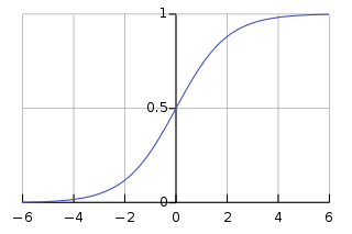
    "An activation function is a normal mathematical function. It takes in one independent variable and gives you some output. There are many activation functions, the one we are going to use is called *sigmoid*. More information about sigmoid could be found [here](https://en.wikipedia.org/wiki/Sigmoid_function). Activation functions define a limit to what will be stored to a neuron. It determines the value to store in the neuron\n",
    "\n",
    "Sigmoid is a mathematical function whose Range is limited to (0,1) but Domain is (-inf,+inf). Sigmoid function is defined as \n",
    "\n",
    "![sigmoid](https://wikimedia.org/api/rest_v1/media/math/render/svg/9537e778e229470d85a68ee0b099c08298a1a3f6) \n",
    "\n",
    "Here is the graph of Sigmoid :\n",
    "\n",
    "![graph](https://upload.wikimedia.org/wikipedia/commons/thumb/8/88/Logistic-curve.svg/320px-Logistic-curve.svg.png)\n",
    "\n",
    "\n",
    "One important thing about Sigmoid is that the derivative of this activation function could be represented in terms of iteself. Try to find it its derivative it will eventually become another combination of sigmoid. Here is the derivative of the Sigmoid :\n",
    "\n",
    "![Imgur](https://i.imgur.com/i1f0wZ7.png)\n",
    "\n",
    "Here is Derivation [click](https://analyticsindiamag.com/wp-content/uploads/2018/01/derivative-sigmoid.jpg)\n",
    "\n",
    "\n",
    "*We need sigmoid's derivative in Gradient Descent Algorithm : So had to find it*\n",
    "\n",
    "The cell below implements sigmoid using numpy. We are using vectorization if you are not familiar with this technique, or with numpy : [Here is a good guide](https://www.safaribooksonline.com/library/view/python-for-data/9781449323592/ch04.html)"
   ]
  },
  {
   "cell_type": "code",
   "execution_count": 4,
   "metadata": {
    "collapsed": true
   },
   "outputs": [],
   "source": [
    "def sigmoid(x, derivative=False):\n",
    "    if derivative:\n",
    "        return x*(1-x)\n",
    "    else:\n",
    "        return 1/(1+np.exp(-x))"
   ]
  },
  {
   "cell_type": "markdown",
   "metadata": {},
   "source": [
    "#### Binary Cross Entropy\n",
    "Binary Cross Entropy is the loss function for our model. Our model will do a binary classification, either 0 or 1 (in reality something close to it). We will use this to calculate how bad our model performs with given inputs.\n",
    "\n",
    "Higher the value returned by this function, Poor is the performance. During our training we would like to minimize this loss. If you want to learn more about cross entropy, [this](https://rdipietro.github.io/friendly-intro-to-cross-entropy-loss/) will be a good read.\n",
    "\n",
    "\n",
    "This is a mathematical representation of the function implemented below : ![Imgur](https://i.imgur.com/1Fykldh.png)\n",
    "\n",
    "\n",
    "Here *y* is a the true vector, *z* is the prediction vector and n is the size of dimension of the vector. We will return a single float indicating the loss of the model.\n",
    "\n",
    "**PLEASE NOTE : THERE IS NO PROBLEM WITH USING log(z) OR log(1-z)**. \n",
    "\n",
    "Log is always defined, because *z* can Never be zero or one as Sigmoid Never gives 0 or 1, It only Aapproaches 0 or 1 as Input Approaches Infinity."
   ]
  },
  {
   "cell_type": "code",
   "execution_count": 5,
   "metadata": {
    "collapsed": true
   },
   "outputs": [],
   "source": [
    "def binary_cross_entropy(yHat, y): # yHat is z in above expression (prediction)\n",
    "    p1 = -np.multiply(y, np.log(yHat)) #y is same as y in above expression (true value)\n",
    "    p2 = -np.multiply((1-y), np.log(1-yHat))\n",
    "    return np.mean(p1+p2)"
   ]
  },
  {
   "cell_type": "markdown",
   "metadata": {},
   "source": [
    "#### Derivative of Binary Cross Entropy\n",
    "\n",
    "As mentioned previously, the above function computes a loss indicating how poor our model is predicting. Well that is  a simple mathematical function, so let's take some help of maths here. We want to minimize that loss. Lower it gets better our model becomes. So we compute its derivative with respect each of the predicted values in the prediction vector.\n",
    "\n",
    "So differentiating above expression with respect to *z* will give :\n",
    "![Imgur](https://i.imgur.com/0KYKaNi.png)\n",
    "\n",
    "You may note that we do not take mean of above derivatives, that is because we want to compute how loss changes with respect to each input. In one time we will feed 5 inputs and we will get 5 predictions each corresponsing to one sample in x_train. (This is called batch Processing although here batch is very small only 5. More info [here](https://visualstudiomagazine.com/articles/2014/08/01/batch-training.aspx))\n",
    "\n",
    "The code snippet below calculate the derivative for us. It will give a [5,1] vector each derivatice for each input we fed."
   ]
  },
  {
   "cell_type": "code",
   "execution_count": 6,
   "metadata": {
    "code_folding": [],
    "collapsed": true
   },
   "outputs": [],
   "source": [
    "def binary_cross_entropy_derivative(yHat, y):\n",
    "    a = np.divide(y,yHat)\n",
    "    b = np.divide((1-y),(1-yHat))\n",
    "    return -a+b"
   ]
  },
  {
   "cell_type": "markdown",
   "metadata": {},
   "source": [
    "#### Creating Weights and Biases\n",
    "To get yourself familiar with these terms. Have a look at [this](http://neuralnetworksanddeeplearning.com/chap1.html). It is highly recommened for those who don't know the structure of neural network. Or else watch Neural Network [Video](https://www.youtube.com/watch?v=aircAruvnKk) by 3Blue1Brown on Youtube.\n",
    "\n",
    "Here we are creating the weights of our neural network. Our neural network will have one hidden layer of two neurons.\n",
    "\n",
    "**weights** is a list of nd-array as with randomly assigned weights values. We will keep them from -0.5 to 0.5 (Slope of sigmoid is steepest in between these intervals. Have a look at graph of derivative of sigmoid).\n",
    "\n",
    "**biases** is also a list of nd-array with all values set to zero. It is safe to set them to zero.\n",
    "\n",
    "**MAKE SURE YOU DO NOT SET WEIGHTS TO ZERO**\n",
    "To break symmetry in the network you need to set random values to weights in network. For more info read [this](https://stats.stackexchange.com/questions/27112/danger-of-setting-all-initial-weights-to-zero-in-backpropagation)"
   ]
  },
  {
   "cell_type": "code",
   "execution_count": 7,
   "metadata": {
    "collapsed": true
   },
   "outputs": [],
   "source": [
    "weights = [np.random.uniform(-0.5, 0.5, (3, 2)), np.random.uniform(-0.5, 0.5, (2, 1))]\n",
    "biases = [np.zeros(2), np.zeros(1)]"
   ]
  },
  {
   "cell_type": "markdown",
   "metadata": {},
   "source": [
    "#### Hyperparameter\n",
    "Hyperparamters are the switches and knobs of any machine learning model. It is the responsiblity of programmer to set them to good values. Setting them incorrectly make may your model never converge (never to reach minima of loss).\n",
    "\n",
    "**epoch** : Number of training iteration we will do.\n",
    "\n",
    "**alpha** : Sometimes called *learning_rate* is the factor that determines how big steps to make while moving towards minima while back-propagation. Higher the value, quicker the steps but too high value may cause it to jump off the minima. Set it wisely a low value will make it converge slowly.\n",
    "\n",
    "**batch_size** : The number of trainging samples to pass in one iteration. Generally depends on your computing power. Here we will pass all x_train at once to each iteration."
   ]
  },
  {
   "cell_type": "code",
   "execution_count": 8,
   "metadata": {
    "collapsed": true
   },
   "outputs": [],
   "source": [
    "epoch = 20000\n",
    "alpha = 1.6\n",
    "batch_size = 5"
   ]
  },
  {
   "cell_type": "markdown",
   "metadata": {},
   "source": [
    "#### Computing the Derivative of weight of Layer 0\n",
    "So now i think it is good to introduce the Gradinent Descent and Back Propagation. Don't go to codes a lot. I will explain what we are doing. So let's begin.. Shall we..!!!\n",
    "\n",
    "**Backpropagation** : It is simple as the name coveys, we will propagate backwards in our neural network, i.e moving from output layer to input layer and we will update the values of our weights and biases to improve our model. but How do we update them?? Introducing Gradient Descent Algorithm.\n",
    "\n",
    "**Gradient Descent** : It is more of a mathematics than Coding, but both go hand in hand, to understand this you need to have some idea of calculus and derivatives. You can read about them on internet. Remembered we created a function that tells how bad our model performs (*binary_cross_entropy is that function see above*). So this function gives us a floating point number. To improve our model we need to decrease this loss. Here comes the maths. If you look closely to compute loss we take into consideration an argument named *yHat* , this is nothing but some matrix multiplications and addition with input and weights and biases (Will talk about it later). So simply we compute the derivative of loss wrt to each input variable and that gives us how quickly loss increase or decreases when the value of that variable is changed. To compute this we use **Chain Rule**. You can read about it on Wikipedia.\n",
    "\n",
    "The code below computes the derivative of loss with respect to weights of layer_0, the one with size of (3,2).\n",
    "Here i have used vectorization of numpy. Please note we are using *mini_batch* (we are feeding all 5 input at once, see_batch size) So we will compute the derivative with each sample input. Hence for each value of weights we will have 5 different derivatives corr. to each input, then we find the mean of that 5 values. Here in my case i had (3,2) weight matrix then my derivative matrix was (3,2,5) then we find the mean along second axis. this will give us a derivative matrix of shape (3,2).\n",
    "\n",
    "Read more about numpy [here](https://docs.scipy.org/doc/numpy-dev/user/quickstart.html).\n",
    "\n",
    "d_1 : is the derivative of logits1 (Will talk in next block)\n",
    "\n",
    "d_2 : is the derivative of logits2 (Will talk in next block)\n",
    "\n",
    "d_3 : is the derivative of entropy computed from *binary_cross_entropy*\n"
   ]
  },
  {
   "cell_type": "code",
   "execution_count": 9,
   "metadata": {
    "collapsed": true
   },
   "outputs": [],
   "source": [
    "def compressed_delta_weight_0(d_1, d_2, d_3):\n",
    "    delta_weights_0 = np.zeros((3, 2))\n",
    "    d_1_split = np.vsplit(d_1, batch_size)\n",
    "    d_2_split = np.vsplit(d_2, batch_size)\n",
    "    d_3_split = np.vsplit(d_3, batch_size)\n",
    "    i = 0\n",
    "    for individual_train_samples in np.vsplit(x_train, batch_size):\n",
    "        temp = d_1_split[i]*d_2_split[i]*d_3_split[i] * \\\n",
    "            weights[1].T*individual_train_samples.T\n",
    "        delta_weights_0 = np.dstack((delta_weights_0, temp))\n",
    "        i = i+1\n",
    "    return np.mean(delta_weights_0, axis=2)"
   ]
  },
  {
   "cell_type": "markdown",
   "metadata": {},
   "source": [
    "#### Computing the Derivative of weights of Layer 1\n",
    "\n",
    "The code below does same as above but with layer1 weights. It computes the gradients and takes the mean about axis=2. You can see that is is less complex than former, it is because this layer is near to output layer and in backpropagation we reach this layer in less steps as compared to former. Hence less codes.\n",
    "\n",
    "The code inside the for loop comes from the popular chain rule (the multiplication part). The arguments to the function are pretty clear."
   ]
  },
  {
   "cell_type": "code",
   "execution_count": 10,
   "metadata": {
    "collapsed": true
   },
   "outputs": [],
   "source": [
    "def compressed_delta_weight_1(d_entropy, d_mlogits1, d_mlogits2):\n",
    "    d_entropy_split = np.vsplit(d_entropy, batch_size)\n",
    "    d_mlogits1_split = np.vsplit(d_mlogits1, batch_size)\n",
    "    i = 0\n",
    "    delta = np.zeros((2,1))\n",
    "    for vals in np.vsplit(d_mlogits2, batch_size):\n",
    "        delta = np.dstack((delta,d_entropy_split[i]*d_mlogits1_split[i]*vals.T))\n",
    "        i=i+1\n",
    "    return np.mean(delta,axis=2)"
   ]
  },
  {
   "cell_type": "markdown",
   "metadata": {},
   "source": [
    "#### Verify how is our model at this Stage\n",
    "Without training let's see how our model predicts the ouputs. It is pretty bad. In the end it will become good Worry Not!!"
   ]
  },
  {
   "cell_type": "code",
   "execution_count": 11,
   "metadata": {},
   "outputs": [
    {
     "name": "stdout",
     "output_type": "stream",
     "text": [
      "Testing on \n",
      " [[0 1 1]\n",
      " [1 1 1]\n",
      " [0 1 0]]\n",
      "Actual Answers are :  [0 1 0]\n",
      "Predicted Answers are :  [0.50564762 0.50466332 0.51113988]\n"
     ]
    }
   ],
   "source": [
    "layer_0 = sigmoid(np.dot(x_test,weights[0]) + biases[0])\n",
    "layer_1 = sigmoid(np.dot(layer_0,weights[1]) + biases[1])\n",
    "print('Testing on \\n',x_test)\n",
    "print('Actual Answers are : ',y_test)\n",
    "print('Predicted Answers are : ',layer_1.reshape(3))"
   ]
  },
  {
   "cell_type": "markdown",
   "metadata": {},
   "source": [
    "#### Main Part : The training loop\n",
    "\n",
    "The complete segment is divided into 3 Parts :\n",
    "\n",
    "**1. Forward Propagation**\n",
    "This step does nothing but feeds the value of input and gets output from the output layer. Let me explain how do we connect weights, biases and inputs to get output.\n",
    "The value in a neuron is determined by : *sigmoid((input x weights) + biases)* => value of next layer.\n",
    "Here you can see that we do not calculate individual values but instead we find the complete layer's value at once. This is vectorization of numpy (Faster than for loops). \n",
    "Then for next layer : *sigmoid((next_layer x weights) + biases)* => value of next_layer2.\n",
    "We follow this pattern unless we reach the last layer.\n",
    "\n",
    "\n",
    "The contents inside of the *sigmoid()* are called logits.\n",
    "\n",
    "After each 1000 iterations we will compute the loss with our function *binary_cross_entropy* and print it.\n",
    "\n",
    "**2. Back Propagation**\n",
    "This step we compute the derivative of each weight and biases in our network. For this we use of helper functions we have created above. Go through the code, it is Simple and Clean. \n",
    "\n",
    "Reading the above you will get to know that we have computed the *biases_delta*, it is relatively easier to calculate as compared to *delta_weights*. There is no super logic, again simple Chain rule helps\n",
    "\n",
    "**3. Update to Variables**\n",
    "This is last step, so now we have gradients of each variable (weights and biases) we need to update it to decrease the loss. A Derivative gived the direction of steepest ascend, that is moving in the side/direction of derivative increases the value of that function, but we need to decrease our loss function that depends on weights and biases. So we move in the direction opposite to that pointed by gradients, for that we take steps negtive to gradients by giving them -ve sign. Now we have a direction to move but the magnitude of movement depends on one of our hyper-parameter called **learning_rate** (here alpha).\n",
    "\n",
    "After we have updated we again run the training and again compute loss and again update, this happens a lot of time depending upon the number of epoch set by user."
   ]
  },
  {
   "cell_type": "code",
   "execution_count": 12,
   "metadata": {},
   "outputs": [
    {
     "name": "stdout",
     "output_type": "stream",
     "text": [
      "Cross Entropy at epoch 0 is 0.6995214876336455\n",
      "Cross Entropy at epoch 1000 is 0.03905352283192724\n",
      "Cross Entropy at epoch 2000 is 0.025169837865809768\n",
      "Cross Entropy at epoch 3000 is 0.020185464863749714\n",
      "Cross Entropy at epoch 4000 is 0.017458653473034384\n",
      "Cross Entropy at epoch 5000 is 0.015683145452460877\n",
      "Cross Entropy at epoch 6000 is 0.014410248228326563\n",
      "Cross Entropy at epoch 7000 is 0.013440090758713908\n",
      "Cross Entropy at epoch 8000 is 0.01266868374636668\n",
      "Cross Entropy at epoch 9000 is 0.012035973508524346\n",
      "Cross Entropy at epoch 10000 is 0.011504568081775935\n",
      "Cross Entropy at epoch 11000 is 0.011049820378825764\n",
      "Cross Entropy at epoch 12000 is 0.010654741516166955\n",
      "Cross Entropy at epoch 13000 is 0.01030719179252389\n",
      "Cross Entropy at epoch 14000 is 0.009998235431216798\n",
      "Cross Entropy at epoch 15000 is 0.00972112947983115\n",
      "Cross Entropy at epoch 16000 is 0.009470677036121897\n",
      "Cross Entropy at epoch 17000 is 0.009242799251939018\n",
      "Cross Entropy at epoch 18000 is 0.009034243749798148\n",
      "Cross Entropy at epoch 19000 is 0.008842380895698188\n"
     ]
    }
   ],
   "source": [
    "for i in range(epoch):\n",
    "    \n",
    "    # Forward Propagation\n",
    "    logits1 = np.matmul(x_train, weights[0]) + biases[0]\n",
    "    mlogit1 = sigmoid(logits1)\n",
    "    logits2 = np.matmul(mlogit1, weights[1]) + biases[1]\n",
    "    mlogit2 = sigmoid(logits2)\n",
    "    if i%1000 == 0:\n",
    "        cross_entropy_loss = binary_cross_entropy(mlogit2, y_train)\n",
    "        print('Cross Entropy at epoch {0} is {1}'.format(i,cross_entropy_loss))\n",
    "\n",
    "\n",
    "    # Back Propagation    \n",
    "    d_entropy = binary_cross_entropy_derivative(mlogit2, y_train)\n",
    "    d_mlogits2 = sigmoid(mlogit2, derivative=True)\n",
    "    d_mlogits1 = sigmoid(mlogit1, derivative=True)\n",
    "\n",
    "    delta_weights_1 = compressed_delta_weight_1(d_entropy, d_mlogits2, d_mlogits1)  \n",
    "    delta_bias_1 = np.mean(d_entropy*d_mlogits2, axis=0) \n",
    "    delta_bias_0 = np.mean(d_entropy*d_mlogits2 *\n",
    "                           d_mlogits1*weights[1].T, axis=0) \n",
    "    delta_weights_0 = compressed_delta_weight_0(\n",
    "        d_mlogits1, d_mlogits2, d_entropy)  \n",
    "\n",
    "    # Lets Update the Values of Weights and Biases  \n",
    "    weights[1] = weights[1] - alpha*delta_weights_1 \n",
    "    weights[0] = weights[0] - alpha*delta_weights_0\n",
    "    biases[0] = biases[0] - alpha*delta_bias_0\n",
    "    biases[1] = biases[1] - alpha*delta_bias_1"
   ]
  },
  {
   "cell_type": "markdown",
   "metadata": {},
   "source": [
    "### Let's Test our network\n",
    "This is the real time, now we need to test our network.\n",
    "\n",
    "It is clearly same as expected, it could be seen that this is not 100% what we wanted but it is very close to what we wanted. This concludes my Notebook."
   ]
  },
  {
   "cell_type": "code",
   "execution_count": 13,
   "metadata": {},
   "outputs": [
    {
     "name": "stdout",
     "output_type": "stream",
     "text": [
      "Testing on \n",
      " [[0 1 1]\n",
      " [1 1 1]\n",
      " [0 1 0]]\n",
      "Actual Answers are :  [0 1 0]\n",
      "Predicted Answers are :  [0.00494261 0.95436655 0.00486861]\n"
     ]
    }
   ],
   "source": [
    "layer_0 = sigmoid(np.dot(x_test,weights[0])+biases[0])\n",
    "layer_1 = sigmoid(np.dot(layer_0,weights[1])+biases[1])\n",
    "\n",
    "print('Testing on \\n',x_test)\n",
    "print('Actual Answers are : ',y_test)\n",
    "print('Predicted Answers are : ',layer_1.reshape(3))"
   ]
  },
  {
   "cell_type": "markdown",
   "metadata": {
    "collapsed": true
   },
   "source": [
    "#### Hope you star and Fork\n",
    "Feel Free to suggest or propose changes. Everything including program or Spellings or English. Happy Machine Learning... :)"
   ]
  }
 ],
 "metadata": {
  "kernelspec": {
   "display_name": "Python 3",
   "language": "python",
   "name": "python3"
  },
  "language_info": {
   "codemirror_mode": {
    "name": "ipython",
    "version": 3
   },
   "file_extension": ".py",
   "mimetype": "text/x-python",
   "name": "python",
   "nbconvert_exporter": "python",
   "pygments_lexer": "ipython3",
   "version": "3.6.3"
  }
 },
 "nbformat": 4,
 "nbformat_minor": 2
}

Done
Changes are welcome