Vanilla encoding and decoding for Homomorphic Encryption

encoding_decoding_ckks_vanilla.ipynb

{
 "cells": [
  {
   "cell_type": "markdown",
   "metadata": {},
   "source": [
    "### Example"
   ]
  },
  {
   "cell_type": "markdown",
   "metadata": {},
   "source": [
    "We will see an example now to better understand what this means.\n",
    "\n",
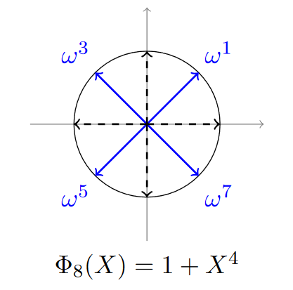
    "Let $M = 8$, $N = \\frac{M}{2}= 4$, $\\Phi_M(X) = X^4 + 1$, and $\\omega = e^{\\frac{2 i \\pi}{8}} = e^{\\frac{i \\pi}{4}}$.\n",
    "Our goal here is to encode the following vectors : $[1, 2, 3, 4]$ and $[-1, -2, -3, -4]$, decode them, add and multiply their polynomial and decode it."
   ]
  },
  {
   "cell_type": "markdown",
   "metadata": {
    "ExecuteTime": {
     "end_time": "2020-05-19T12:37:43.119584Z",
     "start_time": "2020-05-19T12:37:42.812917Z"
    }
   },
   "source": [
    "![title](https://raw.githubusercontent.com/dhuynh95/homomorphic_encryption_intro/master/images/roots.PNG)\n",
    "<center>Roots of $X^4 + 1$ (source : <a href=\"https://heat-project.eu/School/Chris%20Peikert/slides-heat2.pdf\">Cryptography from Rings, HEAT summer school 2016)</a></center>"
   ]
  },
  {
   "cell_type": "markdown",
   "metadata": {},
   "source": [
    "As we saw, in order to decode a polynomial, we simply need to evaluate it on powers of an $M$-th root of unity. Here we choose $\\xi_M = \\omega = e^{\\frac{i \\pi}{4}}$.\n",
    "\n",
    "Once we have $\\xi$ and $M$, we can define both $\\sigma$ and its inverse $\\sigma^{-1}$, respectively the decoding and the encoding."
   ]
  },
  {
   "cell_type": "code",
   "execution_count": 1,
   "metadata": {
    "ExecuteTime": {
     "end_time": "2020-05-23T17:09:55.396205Z",
     "start_time": "2020-05-23T17:09:55.177934Z"
    }
   },
   "outputs": [
    {
     "data": {
      "text/plain": [
       "(0.7071067811865476+0.7071067811865475j)"
      ]
     },
     "execution_count": 1,
     "metadata": {},
     "output_type": "execute_result"
    }
   ],
   "source": [
    "import numpy as np\n",
    "\n",
    "# First we set the parameters\n",
    "M = 8\n",
    "N = M //2\n",
    "\n",
    "# We set xi, which will be used in our computations\n",
    "xi = np.exp(2 * np.pi * 1j / M)\n",
    "xi"
   ]
  },
  {
   "cell_type": "code",
   "execution_count": 2,
   "metadata": {
    "ExecuteTime": {
     "end_time": "2020-05-23T17:09:55.414687Z",
     "start_time": "2020-05-23T17:09:55.402321Z"
    }
   },
   "outputs": [],
   "source": [
    "from numpy.polynomial import Polynomial\n",
    "\n",
    "class CKKSEncoder:\n",
    "    \"\"\"Basic CKKS encoder to encode complex vectors into polynomials.\"\"\"\n",
    "    \n",
    "    def __init__(self, M: int):\n",
    "        \"\"\"Initialization of the encoder for M a power of 2. \n",
    "        \n",
    "        xi, which is an M-th root of unity will, be used as a basis for our computations.\n",
    "        \"\"\"\n",
    "        self.xi = np.exp(2 * np.pi * 1j / M)\n",
    "        self.M = M\n",
    "        \n",
    "    @staticmethod\n",
    "    def vandermonde(xi: np.complex128, M: int) -> np.array:\n",
    "        \"\"\"Computes the Vandermonde matrix from a m-th root of unity.\"\"\"\n",
    "        \n",
    "        N = M //2\n",
    "        matrix = []\n",
    "        # We will generate each row of the matrix\n",
    "        for i in range(N):\n",
    "            # For each row we select a different root\n",
    "            root = xi ** (2 * i + 1)\n",
    "            row = []\n",
    "\n",
    "            # Then we store its powers\n",
    "            for j in range(N):\n",
    "                row.append(root ** j)\n",
    "            matrix.append(row)\n",
    "        return matrix\n",
    "    \n",
    "    def sigma_inverse(self, b: np.array) -> Polynomial:\n",
    "        \"\"\"Encodes the vector b in a polynomial using an M-th root of unity.\"\"\"\n",
    "\n",
    "        # First we create the Vandermonde matrix\n",
    "        A = CKKSEncoder.vandermonde(self.xi, M)\n",
    "\n",
    "        # Then we solve the system\n",
    "        coeffs = np.linalg.solve(A, b)\n",
    "\n",
    "        # Finally we output the polynomial\n",
    "        p = Polynomial(coeffs)\n",
    "        return p\n",
    "\n",
    "    def sigma(self, p: Polynomial) -> np.array:\n",
    "        \"\"\"Decodes a polynomial by applying it to the M-th roots of unity.\"\"\"\n",
    "\n",
    "        outputs = []\n",
    "        N = self.M //2\n",
    "\n",
    "        # We simply apply the polynomial on the roots\n",
    "        for i in range(N):\n",
    "            root = self.xi ** (2 * i + 1)\n",
    "            output = p(root)\n",
    "            outputs.append(output)\n",
    "        return np.array(outputs)"
   ]
  },
  {
   "cell_type": "markdown",
   "metadata": {},
   "source": [
    "Now we can start experimenting with real values, let's first encode a vector and see how it is encoded."
   ]
  },
  {
   "cell_type": "code",
   "execution_count": 3,
   "metadata": {
    "ExecuteTime": {
     "end_time": "2020-05-23T17:09:55.436335Z",
     "start_time": "2020-05-23T17:09:55.420552Z"
    }
   },
   "outputs": [],
   "source": [
    "# First we initialize our encoder\n",
    "encoder = CKKSEncoder(M)"
   ]
  },
  {
   "cell_type": "code",
   "execution_count": 4,
   "metadata": {
    "ExecuteTime": {
     "end_time": "2020-05-23T17:09:55.453314Z",
     "start_time": "2020-05-23T17:09:55.442307Z"
    }
   },
   "outputs": [
    {
     "data": {
      "text/plain": [
       "array([1, 2, 3, 4])"
      ]
     },
     "execution_count": 4,
     "metadata": {},
     "output_type": "execute_result"
    }
   ],
   "source": [
    "b = np.array([1, 2, 3, 4])\n",
    "b"
   ]
  },
  {
   "cell_type": "markdown",
   "metadata": {},
   "source": [
    "Let's encode the vector now."
   ]
  },
  {
   "cell_type": "code",
   "execution_count": 5,
   "metadata": {
    "ExecuteTime": {
     "end_time": "2020-05-23T17:09:55.469589Z",
     "start_time": "2020-05-23T17:09:55.459420Z"
    }
   },
   "outputs": [
    {
     "data": {
      "text/latex": [
       "$x \\mapsto \\text{(2.5+4.440892098500626e-16j)} + (\\text{(-4.996003610813204e-16+0.7071067811865479j)})\\,x + (\\text{(-3.4694469519536176e-16+0.5000000000000003j)})\\,x^{2} + (\\text{(-8.326672684688674e-16+0.7071067811865472j)})\\,x^{3}$"
      ],
      "text/plain": [
       "Polynomial([ 2.50000000e+00+4.44089210e-16j, -4.99600361e-16+7.07106781e-01j,\n",
       "       -3.46944695e-16+5.00000000e-01j, -8.32667268e-16+7.07106781e-01j], domain=[-1,  1], window=[-1,  1])"
      ]
     },
     "execution_count": 5,
     "metadata": {},
     "output_type": "execute_result"
    }
   ],
   "source": [
    "p = encoder.sigma_inverse(b)\n",
    "p"
   ]
  },
  {
   "cell_type": "markdown",
   "metadata": {},
   "source": [
    "Let's see now how we can extract the vector we had initially from the polynomial: "
   ]
  },
  {
   "cell_type": "code",
   "execution_count": 6,
   "metadata": {
    "ExecuteTime": {
     "end_time": "2020-05-23T17:09:55.486646Z",
     "start_time": "2020-05-23T17:09:55.475335Z"
    }
   },
   "outputs": [
    {
     "data": {
      "text/plain": [
       "array([1.-1.11022302e-16j, 2.-4.71844785e-16j, 3.+2.77555756e-17j,\n",
       "       4.+2.22044605e-16j])"
      ]
     },
     "execution_count": 6,
     "metadata": {},
     "output_type": "execute_result"
    }
   ],
   "source": [
    "b_reconstructed = encoder.sigma(p)\n",
    "b_reconstructed"
   ]
  },
  {
   "cell_type": "markdown",
   "metadata": {},
   "source": [
    "We can see that the reconstruction and the initial vector are very close."
   ]
  },
  {
   "cell_type": "code",
   "execution_count": 7,
   "metadata": {
    "ExecuteTime": {
     "end_time": "2020-05-23T17:09:55.507427Z",
     "start_time": "2020-05-23T17:09:55.491379Z"
    }
   },
   "outputs": [
    {
     "data": {
      "text/plain": [
       "6.944442800358888e-16"
      ]
     },
     "execution_count": 7,
     "metadata": {},
     "output_type": "execute_result"
    }
   ],
   "source": [
    "np.linalg.norm(b_reconstructed - b)"
   ]
  },
  {
   "cell_type": "markdown",
   "metadata": {},
   "source": [
    "As stated before, $\\sigma$ is not chosen randomly to encode and decode, but has a lot of nice properties. Among them, $\\sigma$ is an isomorphism, therefore addition and multiplication on polynomials will result in coefficient wise addition and multiplication on the encoded vectors.\n",
    "\n",
    "The homomorphic property of $\\sigma$ is due to the fact that $X^N = 1$ and $\\xi^N = 1$.\n",
    "\n",
    "We can now start to encode several vectors, and see how we can perform homomorphic operations on them and decode it."
   ]
  },
  {
   "cell_type": "code",
   "execution_count": 8,
   "metadata": {
    "ExecuteTime": {
     "end_time": "2020-05-23T17:09:55.519400Z",
     "start_time": "2020-05-23T17:09:55.512068Z"
    }
   },
   "outputs": [],
   "source": [
    "m1 = np.array([1, 2, 3, 4])\n",
    "m2 = np.array([1, -2, 3, -4])"
   ]
  },
  {
   "cell_type": "code",
   "execution_count": 9,
   "metadata": {
    "ExecuteTime": {
     "end_time": "2020-05-23T17:09:55.533113Z",
     "start_time": "2020-05-23T17:09:55.522145Z"
    }
   },
   "outputs": [],
   "source": [
    "p1 = encoder.sigma_inverse(m1)\n",
    "p2 = encoder.sigma_inverse(m2)"
   ]
  },
  {
   "cell_type": "markdown",
   "metadata": {},
   "source": [
    "We can see that addition is pretty straightforward."
   ]
  },
  {
   "cell_type": "code",
   "execution_count": 10,
   "metadata": {
    "ExecuteTime": {
     "end_time": "2020-05-23T17:09:55.554656Z",
     "start_time": "2020-05-23T17:09:55.535927Z"
    }
   },
   "outputs": [
    {
     "data": {
      "text/latex": [
       "$x \\mapsto \\text{(2.0000000000000004+1.1102230246251565e-16j)} + (\\text{(-0.7071067811865477+0.707106781186547j)})\\,x + (\\text{(2.1094237467877966e-15-1.9999999999999996j)})\\,x^{2} + (\\text{(0.7071067811865466+0.707106781186549j)})\\,x^{3}$"
      ],
      "text/plain": [
       "Polynomial([ 2.00000000e+00+1.11022302e-16j, -7.07106781e-01+7.07106781e-01j,\n",
       "        2.10942375e-15-2.00000000e+00j,  7.07106781e-01+7.07106781e-01j], domain=[-1.,  1.], window=[-1.,  1.])"
      ]
     },
     "execution_count": 10,
     "metadata": {},
     "output_type": "execute_result"
    }
   ],
   "source": [
    "p_add = p1 + p2\n",
    "p_add"
   ]
  },
  {
   "cell_type": "markdown",
   "metadata": {},
   "source": [
    "Here as expected, we see that p1 + p2 decodes correctly to $[2, 0, 6, 0]$."
   ]
  },
  {
   "cell_type": "code",
   "execution_count": 11,
   "metadata": {
    "ExecuteTime": {
     "end_time": "2020-05-23T17:09:55.570005Z",
     "start_time": "2020-05-23T17:09:55.559203Z"
    }
   },
   "outputs": [
    {
     "data": {
      "text/plain": [
       "array([2.0000000e+00+3.25176795e-17j, 4.4408921e-16-4.44089210e-16j,\n",
       "       6.0000000e+00+1.11022302e-16j, 4.4408921e-16+3.33066907e-16j])"
      ]
     },
     "execution_count": 11,
     "metadata": {},
     "output_type": "execute_result"
    }
   ],
   "source": [
    "encoder.sigma(p_add)"
   ]
  },
  {
   "cell_type": "markdown",
   "metadata": {},
   "source": [
    "Because when doing multiplication we might have terms whose degree is higher than $N$, we will need to do a modulo operation using $X^N + 1$."
   ]
  },
  {
   "cell_type": "markdown",
   "metadata": {},
   "source": [
    "To perform multiplication, we first need to define the polynomial modulus which we will use."
   ]
  },
  {
   "cell_type": "code",
   "execution_count": 12,
   "metadata": {
    "ExecuteTime": {
     "end_time": "2020-05-23T17:09:55.586175Z",
     "start_time": "2020-05-23T17:09:55.572615Z"
    }
   },
   "outputs": [
    {
     "data": {
      "text/latex": [
       "$x \\mapsto \\text{1.0}\\color{LightGray}{ + \\text{0.0}\\,x}\\color{LightGray}{ + \\text{0.0}\\,x^{2}}\\color{LightGray}{ + \\text{0.0}\\,x^{3}} + \\text{1.0}\\,x^{4}$"
      ],
      "text/plain": [
       "Polynomial([1., 0., 0., 0., 1.], domain=[-1,  1], window=[-1,  1])"
      ]
     },
     "execution_count": 12,
     "metadata": {},
     "output_type": "execute_result"
    }
   ],
   "source": [
    "poly_modulo = Polynomial([1,0,0,0,1])\n",
    "poly_modulo"
   ]
  },
  {
   "cell_type": "markdown",
   "metadata": {},
   "source": [
    "Now we can perform multiplication."
   ]
  },
  {
   "cell_type": "code",
   "execution_count": 13,
   "metadata": {
    "ExecuteTime": {
     "end_time": "2020-05-23T17:09:55.598563Z",
     "start_time": "2020-05-23T17:09:55.588519Z"
    }
   },
   "outputs": [],
   "source": [
    "p_mult = p1 * p2 % poly_modulo"
   ]
  },
  {
   "cell_type": "markdown",
   "metadata": {},
   "source": [
    "Finally if we decode it, we can see that we have the expected result."
   ]
  },
  {
   "cell_type": "code",
   "execution_count": 14,
   "metadata": {
    "ExecuteTime": {
     "end_time": "2020-05-23T17:09:55.614745Z",
     "start_time": "2020-05-23T17:09:55.601665Z"
    }
   },
   "outputs": [
    {
     "data": {
      "text/plain": [
       "array([  1.-8.67361738e-16j,  -4.+6.86950496e-16j,   9.+6.86950496e-16j,\n",
       "       -16.-9.08301212e-15j])"
      ]
     },
     "execution_count": 14,
     "metadata": {},
     "output_type": "execute_result"
    }
   ],
   "source": [
    "encoder.sigma(p_mult)"
   ]
  }
 ],
 "metadata": {
  "kernelspec": {
   "display_name": "Python 3",
   "language": "python",
   "name": "python3"
  },
  "language_info": {
   "codemirror_mode": {
    "name": "ipython",
    "version": 3
   },
   "file_extension": ".py",
   "mimetype": "text/x-python",
   "name": "python",
   "nbconvert_exporter": "python",
   "pygments_lexer": "ipython3",
   "version": "3.8.2"
  },
  "toc": {
   "base_numbering": 1,
   "nav_menu": {},
   "number_sections": true,
   "sideBar": true,
   "skip_h1_title": false,
   "title_cell": "Table of Contents",
   "title_sidebar": "Contents",
   "toc_cell": false,
   "toc_position": {},
   "toc_section_display": true,
   "toc_window_display": false
  }
 },
 "nbformat": 4,
 "nbformat_minor": 4
}