Last active
February 8, 2021 09:54
-
-
Save fohria/21edf9c5be5bd440f0ef652d697ea125 to your computer and use it in GitHub Desktop.
markov stuffs
This file contains bidirectional Unicode text that may be interpreted or compiled differently than what appears below. To review, open the file in an editor that reveals hidden Unicode characters.
Learn more about bidirectional Unicode characters
| { | |
| "cells": [ | |
| { | |
| "cell_type": "markdown", | |
| "metadata": {}, | |
| "source": [ | |
| "# about (hidden) markov models\n", | |
| "\n", | |
| "\n", | |
| "\n", | |
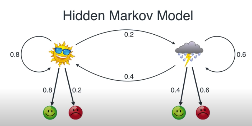
| "this is a hidden markov model. the weather can be sunny or rainy. the weather causes some person to be happy or grumpy. we talk to this person over the phone, so we can only observe their mood and not the weather.\n", | |
| "\n", | |
| "- the weather is our **states**.\n", | |
| "- the moods are our observations or **emissions**\n", | |
| "- numbers are probabilities\n", | |
| "- - weather changes according to a **transition matrix**\n", | |
| "- - emission probabilities (can) differ between states\n", | |
| "\n", | |
| "we can visualise hidden markov models as a water surface; we have some hidden state benath the surface and it causes emissions above the surface. this could be donald duck underwater, using a reed to breathe and the reed makes some random walk. it could also be a whale swimming, and hidden state is either swimming underwater or going up for air so emission would be either nothing or a water cascade. or maybe it could be an iceberg. anyway, water surface.\n", | |
| "\n", | |
| "## table of contents\n", | |
| "\n", | |
| "## markov models\n", | |
| "\n", | |
| "a [markov model](https://en.wikipedia.org/wiki/Markov_model) is a series of states where the future states only depend on the current state, not the history of states. in other words, it's a series of states with the markov property.\n", | |
| "\n", | |
| "the simplest markov model is the **markov chain**. we can see it as a sequence of states, $S$, through discrete time steps:\n", | |
| "\n", | |
| "$$\n", | |
| "S = [s_t, s_{t+1}, s_{t+2}, ... , s_{t+n}]\n", | |
| "$$\n", | |
| "\n", | |
| "### generating a sequence/markov chain\n", | |
| "\n", | |
| "let's generate a weather sequence. python won't like that we are using emojis for the states, so first we've to agree that 🌧 is `0` and ☀️ is `1`.\n", | |
| "\n", | |
| "on any given day, we have the **initial probability** that we get ☀️ with probability $\\dfrac{2}{3}$ and 🌧 with probability $\\dfrac{1}{3}$. we can also call this our **prior** for state/weather." | |
| ] | |
| }, | |
| { | |
| "cell_type": "code", | |
| "execution_count": null, | |
| "metadata": {}, | |
| "outputs": [], | |
| "source": [ | |
| "import numpy as np\n", | |
| "sequence = []\n", | |
| "states = {'rainy': 0, 'sunny': 1}\n", | |
| "init_probs = np.array([1/3, 2/3])\n", | |
| "first_state = np.random.choice(list(states.values()), p=init_probs)\n", | |
| "sequence.append(first_state)" | |
| ] | |
| }, | |
| { | |
| "cell_type": "markdown", | |
| "metadata": {}, | |
| "source": [ | |
| "the next state will be picked according to the transition matrix; the probabilities that we will stay in the current state or *transition* to another state. it's called transition even when we stay in the same state.\n", | |
| "\n", | |
| "> by convention, transition matrix rows correspond to the state at time $t$ while columns correspond to state at time $t+1$. Therefore, rows sum to 1 because it's 100% likely we will transition to the same or some other state. assuming, of course, we have full knowledge.\n", | |
| "\n", | |
| "thusly, row 0 below is the transition probabilities for rain. `(0, 0)` is rain -> rain and `(0, 1)` is rain -> sun." | |
| ] | |
| }, | |
| { | |
| "cell_type": "code", | |
| "execution_count": null, | |
| "metadata": {}, | |
| "outputs": [], | |
| "source": [ | |
| "# remember, 0=rain, 1=sun\n", | |
| "trans_probs = np.array([\n", | |
| " [0.6, 0.4],\n", | |
| " [0.2, 0.8]\n", | |
| "])" | |
| ] | |
| }, | |
| { | |
| "cell_type": "markdown", | |
| "metadata": {}, | |
| "source": [ | |
| "now, every such transition matrix has a **stationary/equilibrium distribution**. meaning, if we generate enough states, we will reach an equilibrium where the probability to be in a certain state becomes fixed. we can show this either by generating lots of states or calculate it analytically.\n", | |
| "\n", | |
| "the analytical solution can be shown, which we won't do here, but we have a python function based on the analytical solution:" | |
| ] | |
| }, | |
| { | |
| "cell_type": "code", | |
| "execution_count": null, | |
| "metadata": {}, | |
| "outputs": [], | |
| "source": [ | |
| "# from functions import equilibrium_distribution # doesnt work when remote\n", | |
| "def equilibrium_distribution(p_transition):\n", | |
| " \"\"\"\n", | |
| " returns the stationary/equilibium distribution for markov model\n", | |
| " transition matrix 'p_transition'\n", | |
| "\n", | |
| " input: p_transition: np.array\n", | |
| " returns: p_eq; np.array\n", | |
| "\n", | |
| " credits: copied from ericmjl; in test.ipynb we discuss maths\n", | |
| " \"\"\"\n", | |
| " n_states = p_transition.shape[0]\n", | |
| " A = np.append(\n", | |
| " arr=p_transition.T - np.eye(n_states),\n", | |
| " values=np.ones(n_states).reshape(1, -1),\n", | |
| " axis=0\n", | |
| " )\n", | |
| " b = np.transpose(np.array([0] * n_states + [1]))\n", | |
| " p_eq = np.linalg.solve(\n", | |
| " a=np.transpose(A).dot(A),\n", | |
| " b=np.transpose(A).dot(b)\n", | |
| " )\n", | |
| " return p_eq\n", | |
| "equilibrium_distribution(trans_probs)" | |
| ] | |
| }, | |
| { | |
| "cell_type": "markdown", | |
| "metadata": {}, | |
| "source": [ | |
| "it gives us the exact values we had as our initial probabilities! that's good. but it actually doesn't matter, we would always reach this equilibrium regardless of what we chose as our initial probabilities, if we just generate a long enough sequence.\n", | |
| "\n", | |
| "shall we do the actual generation now then? yes.\n", | |
| "\n", | |
| "#### multinomial distribution\n", | |
| "\n", | |
| "a [multinomial distribution](https://en.wikipedia.org/wiki/Multinomial_distribution) is a generalization of the binomial distribution. the binomial distribution is repeated flips of a coin. a single flip of a coin is the bernoulli distribution.\n", | |
| "\n", | |
| "for a single event of more than one outcome, i.e. more sides than a coin - for example a die/dice - then it's a categorical distribution. and so finally we get back to multinomial distribution which is, you guessed it! repeated throws of a die, or repeated outcomes of categorical distribution. so each outcome is independent:\n", | |
| "\n", | |
| "> The multinomial distribution models the outcome of n experiments, where the outcome of each trial has a categorical distribution, such as rolling a k-sided dice n times.\n", | |
| "\n", | |
| "ah, and an interesting side note here is:\n", | |
| "\n", | |
| "> In some fields such as natural language processing, categorical and multinomial distributions are synonymous and it is common to speak of a multinomial distribution when a categorical distribution is actually meant.\n", | |
| "\n", | |
| "in pymc3, they say categorical is \"the most general discrete distribution\", whereas multinomial is a form of \"multivariate\" distribution. i'm unsure how they differ/are alike.\n", | |
| "\n", | |
| "we will use scipy to generate values, as pymc3 needs to compile to generate numbers, but perhaps we'll do that later.\n", | |
| "\n", | |
| "#### actually generating then\n", | |
| "\n", | |
| "`scipy.stats.multinomial` works like this. first parameter is `n` or how many dice to throw. the second parameter `p` gives the probabilities for each category. so it will infer from `p` how many sides the die has. below we therefore always set `n=1` as we only want one state each time. and `p` will be a row in the transition matrix, which in our weather example is of length 2.\n", | |
| "\n", | |
| "furthermore, multinomial returns an array with counts of each category. so in our example we will either get back `[0, 1]` or `[1, 0]` where the index indicates what outcome happened. we can therefore use numpy's `argmax` to get that index and thus the state for the current timestep." | |
| ] | |
| }, | |
| { | |
| "cell_type": "code", | |
| "execution_count": null, | |
| "metadata": {}, | |
| "outputs": [], | |
| "source": [ | |
| "from scipy import stats\n", | |
| "\n", | |
| "def generate_markov_sequence(\n", | |
| " transition_matrix, state_count, init_probs = None):\n", | |
| " \"\"\"\n", | |
| " Generate markov chain of length `state_count`\n", | |
| " states are based on rows of `transition_matrix` and first state is\n", | |
| " either from the equilibirum distribution or using `init_probs`\n", | |
| "\n", | |
| " parameters:\n", | |
| " - init_probs: use these probabilities for first state\n", | |
| " - state_count: how many states we want (int)\n", | |
| " - transition_matrix: the transition matrix (np.array)\n", | |
| "\n", | |
| " returns: np.array with length `state_count`\n", | |
| " \"\"\"\n", | |
| "\n", | |
| " if init_probs is None:\n", | |
| " init_probs = equilibrium_distribution(transition_matrix)\n", | |
| " first_state = stats.multinomial.rvs(1, init_probs).argmax()\n", | |
| "\n", | |
| " sequence = [first_state]\n", | |
| " for timestep in range(state_count - 1): # already added first state\n", | |
| " trans_probs = transition_matrix[sequence[-1]]\n", | |
| " next_state = stats.multinomial.rvs(1, trans_probs).argmax()\n", | |
| " sequence.append(next_state)\n", | |
| "\n", | |
| " return np.array(sequence)" | |
| ] | |
| }, | |
| { | |
| "cell_type": "markdown", | |
| "metadata": {}, | |
| "source": [ | |
| "to test the generation and that we get the stationary distribution we generate 10000 states and check the ratio of sunny (1) to rainy (0):" | |
| ] | |
| }, | |
| { | |
| "cell_type": "code", | |
| "execution_count": null, | |
| "metadata": {}, | |
| "outputs": [], | |
| "source": [ | |
| "states = generate_markov_sequence(trans_probs, 10000)\n", | |
| "states.sum() / 10000" | |
| ] | |
| }, | |
| { | |
| "cell_type": "markdown", | |
| "metadata": {}, | |
| "source": [ | |
| "let's also create a small function to pretty print the weather" | |
| ] | |
| }, | |
| { | |
| "cell_type": "code", | |
| "execution_count": null, | |
| "metadata": {}, | |
| "outputs": [], | |
| "source": [ | |
| "def print_weather(states):\n", | |
| " weather = {0: \"🌧\", 1: \"☀️\"}\n", | |
| " weather_states = [weather[state] for state in states]\n", | |
| " print(weather_states)\n", | |
| "states = generate_markov_sequence(trans_probs, 5)\n", | |
| "print_weather(states)" | |
| ] | |
| }, | |
| { | |
| "cell_type": "markdown", | |
| "metadata": {}, | |
| "source": [ | |
| "## hidden markov model\n", | |
| "\n", | |
| "a **hidden markov model** is when each state in the markov sequence has some type of \"emission\". in our case, following [luis](https://github.com/luisguiserrano/hmm), we have the emissions of someone's mood which can be happy 😄 (1) or grumpy 😡 (0).\n", | |
| "\n", | |
| "since these emissions are discrete, we can use the same `multinomial` function from before to create these emissions based on the state sequence we send. the emission probability matrix works like the transition probability matrix in that row 0 is rainy, and in that state we've got 0.6 probability for grumpy and 0.4 probability for happy." | |
| ] | |
| }, | |
| { | |
| "cell_type": "code", | |
| "execution_count": null, | |
| "metadata": {}, | |
| "outputs": [], | |
| "source": [ | |
| "emission_probs = np.array([\n", | |
| " [0.6, 0.4],\n", | |
| " [0.2, 0.8]\n", | |
| "])\n", | |
| "\n", | |
| "def mood_emissions(states, emission_probs):\n", | |
| " \"\"\"\n", | |
| " emit moods for each state in `states`, according to probabilities in\n", | |
| " `emission_probs`\n", | |
| "\n", | |
| " returns: np.array of moods where 0 is grumpy and 1 is happy\n", | |
| " \"\"\"\n", | |
| " emissions = []\n", | |
| " for state in states:\n", | |
| " mood_prob = emission_probs[state]\n", | |
| " mood = stats.multinomial.rvs(1, mood_prob).argmax()\n", | |
| " emissions.append(mood)\n", | |
| "\n", | |
| " return np.array(emissions)" | |
| ] | |
| }, | |
| { | |
| "cell_type": "markdown", | |
| "metadata": {}, | |
| "source": [ | |
| "let's test it with the short state sequence we already have in memory:" | |
| ] | |
| }, | |
| { | |
| "cell_type": "code", | |
| "execution_count": null, | |
| "metadata": {}, | |
| "outputs": [], | |
| "source": [ | |
| "def print_moods(emissions):\n", | |
| " moods = {0: \"😡\", 1: \"😄\"}\n", | |
| " mood_faces = [moods[emission] for emission in emissions]\n", | |
| " print(mood_faces)\n", | |
| "\n", | |
| "emissions = mood_emissions(states, emission_probs)\n", | |
| "print_weather(states)\n", | |
| "print_moods(emissions)" | |
| ] | |
| }, | |
| { | |
| "cell_type": "markdown", | |
| "metadata": {}, | |
| "source": [ | |
| "## finding the hidden states\n", | |
| "\n", | |
| "now, say we call our friend over a bunch of days and observe their mood. how do we find out what the weather was like over there?\n", | |
| "\n", | |
| "if we know all the transition probabilities and emission probabilities, then we can use the **viterbi algorithm** to calculate the chain of most likely hidden states (weather). simply put it just starts from the first state, calculates the probabilities of every combination at every step and then selects the path that has the highest probability.\n", | |
| "\n", | |
| "> sidenote: see [here](https://www.maths.lancs.ac.uk/~fearnhea/GTP/GTP_Slides.pdf) for some slides on viterbi vs mcmc and the paper scott 2002 for additional info.\n", | |
| "\n", | |
| "however, if we do not know the transition probabilities and/or dont know the emission probabilities, we need to infer these. so let's use pymc3.\n", | |
| "\n", | |
| "## pymc3 inference of HMM\n", | |
| "\n", | |
| "### step 1: loglikelihood functions\n", | |
| "\n", | |
| "there's no built in distribution for (hidden) markov models, so we need to create our own by extending a built in distribution. we're basing our class on [ericmjl's implementation](https://ericmjl.github.io/essays-on-data-science/machine-learning/markov-models/#hmm-states-distribution) of [hstrey's original](https://github.com/hstrey/Hidden-Markov-Models-pymc3/blob/master/Multi-State%20HMM.ipynb).\n", | |
| "\n", | |
| "> sidenote: for future reference [this](https://sidravi1.github.io/blog/2019/01/25/heirarchical-hidden-markov-model) also looks promising for inspiration/alternate implementation. oh and there's an actual pymc3 plugin called [pymc3-hmm](https://github.com/AmpersandTV/pymc3-hmm). and some [troubleshooting](https://discourse.pymc.io/t/theano-scan-and-pm-model-are-strangely-incompatible/3298/2)" | |
| ] | |
| }, | |
| { | |
| "cell_type": "code", | |
| "execution_count": null, | |
| "metadata": {}, | |
| "outputs": [], | |
| "source": [ | |
| "# to get sampling work on macos we need a workaround that doesnt work\n", | |
| "# https://github.com/pymc-devs/pymc3/issues/3844\n", | |
| "\n", | |
| "import pymc3 as pm\n", | |
| "import theano.tensor as tt\n", | |
| "\n", | |
| "\n", | |
| "class HMMStates(pm.Categorical):\n", | |
| " def __init__(self, p_transition, p_equilibrium, n_states, *args, **kwargs):\n", | |
| " super(pm.Categorical, self).__init__(*args, **kwargs)\n", | |
| " self.p_transition = p_transition\n", | |
| " self.p_equilibrium = p_equilibrium\n", | |
| " self.k = n_states\n", | |
| " self.mode = tt.cast(0, dtype = 'int64')\n", | |
| "\n", | |
| " def logp(self, x):\n", | |
| " # x are the observations/states\n", | |
| " p_eq = self.p_equilibrium\n", | |
| " p_tr = self.p_transition[x[:-1]]\n", | |
| "\n", | |
| " init_state_logp = pm.Categorical.dist(p_eq).logp(x[0])\n", | |
| "\n", | |
| " x_i = x[1:]\n", | |
| " ou_like = pm.Categorical.dist(p_tr).logp(x_i)\n", | |
| " transition_logp = tt.sum(ou_like)\n", | |
| " return init_state_logp + transition_logp" | |
| ] | |
| }, | |
| { | |
| "cell_type": "markdown", | |
| "metadata": {}, | |
| "source": [ | |
| "### equilibrium distribution\n", | |
| "\n", | |
| "we also need a pymc3/theano function for solving the equilibrium distribution" | |
| ] | |
| }, | |
| { | |
| "cell_type": "code", | |
| "execution_count": null, | |
| "metadata": {}, | |
| "outputs": [], | |
| "source": [ | |
| "import theano.tensor.slinalg as sla # theano-wrapped scipy linalg\n", | |
| "\n", | |
| "def solve_equilibrium(n_states, p_transition):\n", | |
| " A = tt.dmatrix('A')\n", | |
| " A = tt.eye(n_states) - p_transition + tt.ones(shape = (n_states, n_states))\n", | |
| " p_equilibrium = pm.Deterministic(\n", | |
| " \"p_equilibrium\", sla.solve(A.T, tt.ones(shape = n_states))\n", | |
| " )\n", | |
| "\n", | |
| " return p_equilibrium" | |
| ] | |
| }, | |
| { | |
| "cell_type": "markdown", | |
| "metadata": {}, | |
| "source": [ | |
| "### the actual probabilistic model\n", | |
| "\n", | |
| "what kind of prior distribution is good for the transition probability matrix? well, it's a **dirichlet distribution**. why? they're generalisation of beta distribution. the metaphor is breaking a stick into potentially infinitely many parts.\n", | |
| "\n", | |
| "#### TODO! better understand dirichlet\n", | |
| "\n", | |
| "i've seen at least half a lecture on it and it kind of made sense at the time but i haven't grasped it fully yet, especially not why it's a good prior for this matrix.\n", | |
| "\n", | |
| "> note; see the dirichlet note in bear/locally on svarten. also see reviews.py in this folder for some code playing with 1blue3brown binomial example.\n", | |
| "\n", | |
| "maybe it has something to do with that each row in the matrix has to sum up to 1 for the probability, and the breaking of the stick has the same property?\n", | |
| "\n", | |
| "#### constructing the model\n", | |
| "\n", | |
| "lets get more than 5-6 states so we have a chance of getting good results" | |
| ] | |
| }, | |
| { | |
| "cell_type": "code", | |
| "execution_count": null, | |
| "metadata": {}, | |
| "outputs": [], | |
| "source": [ | |
| "states = generate_markov_sequence(trans_probs, 1000)" | |
| ] | |
| }, | |
| { | |
| "cell_type": "code", | |
| "execution_count": null, | |
| "metadata": {}, | |
| "outputs": [], | |
| "source": [ | |
| "n_states = 2\n", | |
| "with pm.Model() as model:\n", | |
| " p_transition = pm.Dirichlet(\n", | |
| " \"p_transition\",\n", | |
| " a = tt.ones((n_states, n_states)) * 4, # not sure what the 4 is\n", | |
| " shape = (n_states, n_states)\n", | |
| " )\n", | |
| "\n", | |
| " p_equilibrium = solve_equilibrium(n_states, p_transition)\n", | |
| "\n", | |
| " obs_states = HMMStates(\n", | |
| " \"states\",\n", | |
| " p_transition = p_transition,\n", | |
| " p_equilibrium = p_equilibrium,\n", | |
| " n_states = n_states,\n", | |
| " observed = states.astype('float') # not sure why we want this but ok\n", | |
| " )" | |
| ] | |
| }, | |
| { | |
| "cell_type": "markdown", | |
| "metadata": {}, | |
| "source": [ | |
| "and then sample it:" | |
| ] | |
| }, | |
| { | |
| "cell_type": "code", | |
| "execution_count": null, | |
| "metadata": {}, | |
| "outputs": [], | |
| "source": [ | |
| "import pymc3 as pm\n", | |
| "\n", | |
| "with model:\n", | |
| " trace = pm.sample(2000)" | |
| ] | |
| }, | |
| { | |
| "cell_type": "markdown", | |
| "metadata": {}, | |
| "source": [ | |
| "and plot it:" | |
| ] | |
| }, | |
| { | |
| "cell_type": "code", | |
| "execution_count": null, | |
| "metadata": {}, | |
| "outputs": [], | |
| "source": [ | |
| "import arviz as az\n", | |
| "az_trace = az.from_pymc3(trace, model=model)\n", | |
| "print(az.summary(az_trace))\n", | |
| "print(trans_probs)\n", | |
| "az.plot_forest(az_trace, var_names=[\"p_transition\"])" | |
| ] | |
| }, | |
| { | |
| "cell_type": "markdown", | |
| "metadata": {}, | |
| "source": [ | |
| "woho! we can recover the transition matrix pretty well with 1000 states!\n", | |
| "\n", | |
| "## pymc3 inference for emissions\n", | |
| "\n", | |
| "we will again base this on [ericmjl's implementation](https://ericmjl.github.io/essays-on-data-science/machine-learning/markov-models/#hmm-with-gaussian-emissions) but adapt it to use categorical emissions, so it'll actually look more like the `HMMStates` class." | |
| ] | |
| }, | |
| { | |
| "cell_type": "code", | |
| "execution_count": null, | |
| "metadata": {}, | |
| "outputs": [], | |
| "source": [ | |
| "class MoodEmissions(pm.Categorical):\n", | |
| "\n", | |
| " def __init__(self, states, emission_probs, n_moods, *args, **kwargs):\n", | |
| " super(pm.Categorical, self).__init__(*args, **kwargs)\n", | |
| " self.states = states\n", | |
| " self.emission_probs = emission_probs\n", | |
| " self.k = n_moods\n", | |
| " self.mode = tt.cast(0, dtype = 'int64')\n", | |
| "\n", | |
| " def logp(self, x):\n", | |
| " # x are the observations/moods/emissions\n", | |
| " states = self.states\n", | |
| " probs = self.emission_probs[states]\n", | |
| " out_like = pm.Categorical.dist(probs).logp(x)\n", | |
| " return tt.sum(out_like)" | |
| ] | |
| }, | |
| { | |
| "cell_type": "markdown", | |
| "metadata": {}, | |
| "source": [ | |
| "then we use a dirichlet prior for this one as well and just to check our class works we'll start with known states." | |
| ] | |
| }, | |
| { | |
| "cell_type": "code", | |
| "execution_count": null, | |
| "metadata": {}, | |
| "outputs": [], | |
| "source": [ | |
| "mood_probs = emission_probs.copy()\n", | |
| "moods = mood_emissions(states, mood_probs)\n", | |
| "\n", | |
| "n_moods = 2\n", | |
| "\n", | |
| "with pm.Model() as mood_model:\n", | |
| " p_emissions = pm.Dirichlet(\n", | |
| " \"p_emissions\",\n", | |
| " a = tt.ones((n_moods, n_moods)),\n", | |
| " shape = (n_moods, n_moods)\n", | |
| " )\n", | |
| "\n", | |
| " obs = MoodEmissions(\n", | |
| " \"emissions\",\n", | |
| " states = states,\n", | |
| " emission_probs = p_emissions,\n", | |
| " n_moods = n_moods,\n", | |
| " observed = moods.astype('float')\n", | |
| " )" | |
| ] | |
| }, | |
| { | |
| "cell_type": "markdown", | |
| "metadata": {}, | |
| "source": [ | |
| "aaaand lets try it out!" | |
| ] | |
| }, | |
| { | |
| "cell_type": "code", | |
| "execution_count": null, | |
| "metadata": {}, | |
| "outputs": [], | |
| "source": [ | |
| "with mood_model:\n", | |
| " mood_trace = pm.sample(2000) #, target_accept = 0.9)" | |
| ] | |
| }, | |
| { | |
| "cell_type": "markdown", | |
| "metadata": {}, | |
| "source": [ | |
| "plot/summary it:" | |
| ] | |
| }, | |
| { | |
| "cell_type": "code", | |
| "execution_count": null, | |
| "metadata": {}, | |
| "outputs": [], | |
| "source": [ | |
| "az_mood_trace = az.from_pymc3(mood_trace, model=mood_model)\n", | |
| "print(az.summary(az_mood_trace))\n", | |
| "print(mood_probs)" | |
| ] | |
| }, | |
| { | |
| "cell_type": "markdown", | |
| "metadata": {}, | |
| "source": [ | |
| "that also works nicely for 1000 moods!\n", | |
| "\n", | |
| "## pymc3 inference with HMM + emissions\n", | |
| "\n", | |
| "we have all the components needed so now let's create our combined model:" | |
| ] | |
| }, | |
| { | |
| "cell_type": "code", | |
| "execution_count": null, | |
| "metadata": {}, | |
| "outputs": [], | |
| "source": [ | |
| "n_states = 2\n", | |
| "n_moods = 2\n", | |
| "\n", | |
| "with pm.Model() as combo_model:\n", | |
| " # hmm transition matrix prior\n", | |
| " p_transition = pm.Dirichlet(\n", | |
| " \"trans_probs\",\n", | |
| " a = tt.ones((n_states, n_states)),\n", | |
| " shape = (n_states, n_states)\n", | |
| " )\n", | |
| "\n", | |
| " # equilibirum state for transition matrix\n", | |
| " p_equilibrium = solve_equilibrium(n_states, p_transition)\n", | |
| "\n", | |
| " # hmm states\n", | |
| " hmm_states = HMMStates(\n", | |
| " \"hmm_states\",\n", | |
| " p_transition = p_transition,\n", | |
| " p_equilibrium = p_equilibrium,\n", | |
| " n_states = n_states,\n", | |
| " shape = (len(moods),)\n", | |
| " )\n", | |
| "\n", | |
| " # prior for mood emission matrix\n", | |
| " p_emission = pm.Dirichlet(\n", | |
| " \"emission_probs\",\n", | |
| " a = tt.ones((n_moods, n_moods)),\n", | |
| " shape = (n_moods, n_moods)\n", | |
| " )\n", | |
| "\n", | |
| " obs = MoodEmissions(\n", | |
| " \"mood_emissions\",\n", | |
| " states = hmm_states,\n", | |
| " emission_probs = p_emission,\n", | |
| " n_moods = n_moods,\n", | |
| " observed = moods.astype('float')\n", | |
| " )" | |
| ] | |
| }, | |
| { | |
| "cell_type": "markdown", | |
| "metadata": {}, | |
| "source": [ | |
| "sample it!" | |
| ] | |
| }, | |
| { | |
| "cell_type": "code", | |
| "execution_count": null, | |
| "metadata": {}, | |
| "outputs": [], | |
| "source": [ | |
| "with combo_model:\n", | |
| " combo_trace = pm.sample(3000, nuts={'target_accept':0.95}, cores=4)" | |
| ] | |
| }, | |
| { | |
| "cell_type": "code", | |
| "execution_count": null, | |
| "metadata": {}, | |
| "outputs": [], | |
| "source": [ | |
| "az_combo_trace = az.from_pymc3(combo_trace, model=combo_model)\n", | |
| "print(az.summary(az_combo_trace, var_names=['trans_probs', 'emission_probs']))\n", | |
| "az.plot_forest(az_combo_trace, var_names=['emission_probs'])" | |
| ] | |
| }, | |
| { | |
| "cell_type": "markdown", | |
| "metadata": {}, | |
| "source": [ | |
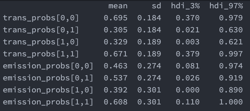
| "results from a run for future reference:\n", | |
| "\n", | |
| "\n", | |
| "## outstanding questions\n", | |
| "\n", | |
| "- it's interesting how trans_probs are all off by ish 0.1 and look like they've moved towards equilibrium. i'm not sure if that's what has happened but it certainly feels like that's what's happened. can we confirm in some way?\n", | |
| "- how does dirichlet work and how is it made into a matrix prior?\n", | |
| "- why does `emission_probs` in combo model give reversed values for 0,1 and 0,0?\n", | |
| " - WELL, looking at it again jan42021 i don't think that's true. emission probs for rainy (`[0,0]` and `[0,1]`) is `0.4` and `0.6` respectively (check hmm_weather image), and in the current run (image above) we see that they're almost there, but we could also almost say its 0.5/0.5 perhaps because they're so close to each other to begin with. for sunny days the real values are farther apart (0.2 and 0.8) so we see that trend here, though hdi range is too big to say anything for sure, but at least we see that (1,0) goes from 0-0.9 (should be 0.2) and (1,1) goes from 0.1-1 when it should be 0.8 so it's kiiind of correct. it's just very uncertain.\n", | |
| "- can we improve results? they're not great at the moment.\n", | |
| "- - perhaps by figuring out how to use the `pymc3-hmm` library?\n", | |
| "\n", | |
| "## additional info/extensions\n", | |
| "\n", | |
| "the following is not relevant to our work (yet).\n", | |
| "\n", | |
| "if emissions depend on previous emissions, they are **autoregressive emissions**. they are common in time series modelling, but since they depend on previous values they're by definition no longer markov: [https://en.wikipedia.org/wiki/Autoregressive_model](https://en.wikipedia.org/wiki/Autoregressive_model)\n", | |
| "\n", | |
| "more info about using pymc3 for such emissions [here](https://ericmjl.github.io/essays-on-data-science/machine-learning/markov-models/)\n", | |
| "\n", | |
| "### what's REALLY interesting about autoregressive HMM\n", | |
| "\n", | |
| "> - **autoregressive** HMM; emission at time $t$ depends on emission from previous time step(s) $t-1, t-2, ..., t-t$\n", | |
| ">\n", | |
| "> $$y_t|s_t \\sim Dist(f(y_{t-1}, \\theta_t))$$\n", | |
| "\n", | |
| "and that we can expand this concept into RNNs:\n", | |
| "\n", | |
| "> Bonus point: your data don't necessarily have to be single dimensional; they can be multidimensional too! As long as you write the $f(y_{t−1}, \\theta_t)$ in a fashion that handles y that are multidimensional, you're golden! Moreover, you can also write the function f to be any function you like. The function f doesn't have to be a linear function (like we did); it can instead be a neural network if you so choose, thus giving you a natural progression from Markov models to **Recurrent Neural Networks**. That, however, is out of scope for this essay." | |
| ] | |
| } | |
| ], | |
| "metadata": { | |
| "jupytext": { | |
| "cell_metadata_filter": "-all", | |
| "main_language": "python", | |
| "notebook_metadata_filter": "-all" | |
| } | |
| }, | |
| "nbformat": 4, | |
| "nbformat_minor": 4 | |
| } |
Sign up for free
to join this conversation on GitHub.
Already have an account?
Sign in to comment