Created
November 10, 2020 11:52
-
-
Save ritog/06c97e45aed6b73c514feaa39b231f0c to your computer and use it in GitHub Desktop.
MIT_S191_Lab1_Part1_TensorFlow.ipynb
This file contains bidirectional Unicode text that may be interpreted or compiled differently than what appears below. To review, open the file in an editor that reveals hidden Unicode characters.
Learn more about bidirectional Unicode characters
| { | |
| "nbformat": 4, | |
| "nbformat_minor": 0, | |
| "metadata": { | |
| "colab": { | |
| "name": "MIT_S191_Lab1_Part1_TensorFlow.ipynb", | |
| "provenance": [], | |
| "collapsed_sections": [ | |
| "WBk0ZDWY-ff8" | |
| ], | |
| "include_colab_link": true | |
| }, | |
| "kernelspec": { | |
| "name": "python3", | |
| "display_name": "Python 3" | |
| }, | |
| "accelerator": "GPU" | |
| }, | |
| "cells": [ | |
| { | |
| "cell_type": "markdown", | |
| "metadata": { | |
| "id": "view-in-github", | |
| "colab_type": "text" | |
| }, | |
| "source": [ | |
| "<a href=\"https://colab.research.google.com/gist/ghosh-r/06c97e45aed6b73c514feaa39b231f0c/mit_s191_lab1_part1_tensorflow.ipynb\" target=\"_parent\"><img src=\"https://colab.research.google.com/assets/colab-badge.svg\" alt=\"Open In Colab\"/></a>" | |
| ] | |
| }, | |
| { | |
| "cell_type": "markdown", | |
| "metadata": { | |
| "id": "WBk0ZDWY-ff8" | |
| }, | |
| "source": [ | |
| "<table align=\"center\">\n", | |
| " <td align=\"center\"><a target=\"_blank\" href=\"http://introtodeeplearning.com\">\n", | |
| " <img src=\"http://introtodeeplearning.com/images/colab/mit.png\" style=\"padding-bottom:5px;\" />\n", | |
| " Visit MIT Deep Learning</a></td>\n", | |
| " <td align=\"center\"><a target=\"_blank\" href=\"https://colab.research.google.com/github/aamini/introtodeeplearning/blob/master/lab1/Part1_TensorFlow.ipynb\">\n", | |
| " <img src=\"http://introtodeeplearning.com/images/colab/colab.png?v2.0\" style=\"padding-bottom:5px;\" />Run in Google Colab</a></td>\n", | |
| " <td align=\"center\"><a target=\"_blank\" href=\"https://github.com/aamini/introtodeeplearning/blob/master/lab1/Part1_TensorFlow.ipynb\">\n", | |
| " <img src=\"http://introtodeeplearning.com/images/colab/github.png\" height=\"70px\" style=\"padding-bottom:5px;\" />View Source on GitHub</a></td>\n", | |
| "</table>\n", | |
| "\n", | |
| "# Copyright Information\n" | |
| ] | |
| }, | |
| { | |
| "cell_type": "code", | |
| "metadata": { | |
| "id": "3eI6DUic-6jo" | |
| }, | |
| "source": [ | |
| "# Copyright 2020 MIT 6.S191 Introduction to Deep Learning. All Rights Reserved.\n", | |
| "# \n", | |
| "# Licensed under the MIT License. You may not use this file except in compliance\n", | |
| "# with the License. Use and/or modification of this code outside of 6.S191 must\n", | |
| "# reference:\n", | |
| "#\n", | |
| "# © MIT 6.S191: Introduction to Deep Learning\n", | |
| "# http://introtodeeplearning.com\n", | |
| "#" | |
| ], | |
| "execution_count": null, | |
| "outputs": [] | |
| }, | |
| { | |
| "cell_type": "markdown", | |
| "metadata": { | |
| "id": "57knM8jrYZ2t" | |
| }, | |
| "source": [ | |
| "# Lab 1: Intro to TensorFlow and Music Generation with RNNs\n", | |
| "\n", | |
| "In this lab, you'll get exposure to using TensorFlow and learn how it can be used for solving deep learning tasks. Go through the code and run each cell. Along the way, you'll encounter several ***TODO*** blocks -- follow the instructions to fill them out before running those cells and continuing.\n", | |
| "\n", | |
| "\n", | |
| "# Part 1: Intro to TensorFlow\n", | |
| "\n", | |
| "## 0.1 Install TensorFlow\n", | |
| "\n", | |
| "TensorFlow is a software library extensively used in machine learning. Here we'll learn how computations are represented and how to define a simple neural network in TensorFlow. For all the labs in 6.S191 2020, we'll be using the latest version of TensorFlow, TensorFlow 2, which affords great flexibility and the ability to imperatively execute operations, just like in Python. You'll notice that TensorFlow 2 is quite similar to Python in its syntax and imperative execution. Let's install TensorFlow and a couple of dependencies.\n" | |
| ] | |
| }, | |
| { | |
| "cell_type": "code", | |
| "metadata": { | |
| "id": "LkaimNJfYZ2w", | |
| "outputId": "01665ca0-9b25-4bad-cba4-1a6efcb336e7", | |
| "colab": { | |
| "base_uri": "https://localhost:8080/" | |
| } | |
| }, | |
| "source": [ | |
| "%tensorflow_version 2.x\n", | |
| "import tensorflow as tf\n", | |
| "\n", | |
| "# Download and import the MIT 6.S191 package\n", | |
| "!pip install mitdeeplearning\n", | |
| "import mitdeeplearning as mdl\n", | |
| "\n", | |
| "import numpy as np\n", | |
| "import matplotlib.pyplot as plt" | |
| ], | |
| "execution_count": 1, | |
| "outputs": [ | |
| { | |
| "output_type": "stream", | |
| "text": [ | |
| "Collecting mitdeeplearning\n", | |
| "\u001b[?25l Downloading https://files.pythonhosted.org/packages/8b/3b/b9174b68dc10832356d02a2d83a64b43a24f1762c172754407d22fc8f960/mitdeeplearning-0.1.2.tar.gz (2.1MB)\n", | |
| "\r\u001b[K |▏ | 10kB 24.5MB/s eta 0:00:01\r\u001b[K |▎ | 20kB 25.5MB/s eta 0:00:01\r\u001b[K |▌ | 30kB 18.3MB/s eta 0:00:01\r\u001b[K |▋ | 40kB 13.3MB/s eta 0:00:01\r\u001b[K |▉ | 51kB 12.2MB/s eta 0:00:01\r\u001b[K |█ | 61kB 11.5MB/s eta 0:00:01\r\u001b[K |█ | 71kB 11.1MB/s eta 0:00:01\r\u001b[K |█▎ | 81kB 11.2MB/s eta 0:00:01\r\u001b[K |█▍ | 92kB 10.3MB/s eta 0:00:01\r\u001b[K |█▋ | 102kB 10.3MB/s eta 0:00:01\r\u001b[K |█▊ | 112kB 10.3MB/s eta 0:00:01\r\u001b[K |█▉ | 122kB 10.3MB/s eta 0:00:01\r\u001b[K |██ | 133kB 10.3MB/s eta 0:00:01\r\u001b[K |██▏ | 143kB 10.3MB/s eta 0:00:01\r\u001b[K |██▍ | 153kB 10.3MB/s eta 0:00:01\r\u001b[K |██▌ | 163kB 10.3MB/s eta 0:00:01\r\u001b[K |██▊ | 174kB 10.3MB/s eta 0:00:01\r\u001b[K |██▉ | 184kB 10.3MB/s eta 0:00:01\r\u001b[K |███ | 194kB 10.3MB/s eta 0:00:01\r\u001b[K |███▏ | 204kB 10.3MB/s eta 0:00:01\r\u001b[K |███▎ | 215kB 10.3MB/s eta 0:00:01\r\u001b[K |███▌ | 225kB 10.3MB/s eta 0:00:01\r\u001b[K |███▋ | 235kB 10.3MB/s eta 0:00:01\r\u001b[K |███▊ | 245kB 10.3MB/s eta 0:00:01\r\u001b[K |████ | 256kB 10.3MB/s eta 0:00:01\r\u001b[K |████ | 266kB 10.3MB/s eta 0:00:01\r\u001b[K |████▎ | 276kB 10.3MB/s eta 0:00:01\r\u001b[K |████▍ | 286kB 10.3MB/s eta 0:00:01\r\u001b[K |████▋ | 296kB 10.3MB/s eta 0:00:01\r\u001b[K |████▊ | 307kB 10.3MB/s eta 0:00:01\r\u001b[K |████▉ | 317kB 10.3MB/s eta 0:00:01\r\u001b[K |█████ | 327kB 10.3MB/s eta 0:00:01\r\u001b[K |█████▏ | 337kB 10.3MB/s eta 0:00:01\r\u001b[K |█████▍ | 348kB 10.3MB/s eta 0:00:01\r\u001b[K |█████▌ | 358kB 10.3MB/s eta 0:00:01\r\u001b[K |█████▋ | 368kB 10.3MB/s eta 0:00:01\r\u001b[K |█████▉ | 378kB 10.3MB/s eta 0:00:01\r\u001b[K |██████ | 389kB 10.3MB/s eta 0:00:01\r\u001b[K |██████▏ | 399kB 10.3MB/s eta 0:00:01\r\u001b[K |██████▎ | 409kB 10.3MB/s eta 0:00:01\r\u001b[K |██████▌ | 419kB 10.3MB/s eta 0:00:01\r\u001b[K |██████▋ | 430kB 10.3MB/s eta 0:00:01\r\u001b[K |██████▊ | 440kB 10.3MB/s eta 0:00:01\r\u001b[K |███████ | 450kB 10.3MB/s eta 0:00:01\r\u001b[K |███████ | 460kB 10.3MB/s eta 0:00:01\r\u001b[K |███████▎ | 471kB 10.3MB/s eta 0:00:01\r\u001b[K |███████▍ | 481kB 10.3MB/s eta 0:00:01\r\u001b[K |███████▌ | 491kB 10.3MB/s eta 0:00:01\r\u001b[K |███████▊ | 501kB 10.3MB/s eta 0:00:01\r\u001b[K |███████▉ | 512kB 10.3MB/s eta 0:00:01\r\u001b[K |████████ | 522kB 10.3MB/s eta 0:00:01\r\u001b[K |████████▏ | 532kB 10.3MB/s eta 0:00:01\r\u001b[K |████████▍ | 542kB 10.3MB/s eta 0:00:01\r\u001b[K |████████▌ | 552kB 10.3MB/s eta 0:00:01\r\u001b[K |████████▋ | 563kB 10.3MB/s eta 0:00:01\r\u001b[K |████████▉ | 573kB 10.3MB/s eta 0:00:01\r\u001b[K |█████████ | 583kB 10.3MB/s eta 0:00:01\r\u001b[K |█████████▏ | 593kB 10.3MB/s eta 0:00:01\r\u001b[K |█████████▎ | 604kB 10.3MB/s eta 0:00:01\r\u001b[K |█████████▍ | 614kB 10.3MB/s eta 0:00:01\r\u001b[K |█████████▋ | 624kB 10.3MB/s eta 0:00:01\r\u001b[K |█████████▊ | 634kB 10.3MB/s eta 0:00:01\r\u001b[K |██████████ | 645kB 10.3MB/s eta 0:00:01\r\u001b[K |██████████ | 655kB 10.3MB/s eta 0:00:01\r\u001b[K |██████████▎ | 665kB 10.3MB/s eta 0:00:01\r\u001b[K |██████████▍ | 675kB 10.3MB/s eta 0:00:01\r\u001b[K |██████████▌ | 686kB 10.3MB/s eta 0:00:01\r\u001b[K |██████████▊ | 696kB 10.3MB/s eta 0:00:01\r\u001b[K |██████████▉ | 706kB 10.3MB/s eta 0:00:01\r\u001b[K |███████████ | 716kB 10.3MB/s eta 0:00:01\r\u001b[K |███████████▏ | 727kB 10.3MB/s eta 0:00:01\r\u001b[K |███████████▎ | 737kB 10.3MB/s eta 0:00:01\r\u001b[K |███████████▌ | 747kB 10.3MB/s eta 0:00:01\r\u001b[K |███████████▋ | 757kB 10.3MB/s eta 0:00:01\r\u001b[K |███████████▉ | 768kB 10.3MB/s eta 0:00:01\r\u001b[K |████████████ | 778kB 10.3MB/s eta 0:00:01\r\u001b[K |████████████ | 788kB 10.3MB/s eta 0:00:01\r\u001b[K |████████████▎ | 798kB 10.3MB/s eta 0:00:01\r\u001b[K |████████████▍ | 808kB 10.3MB/s eta 0:00:01\r\u001b[K |████████████▋ | 819kB 10.3MB/s eta 0:00:01\r\u001b[K |████████████▊ | 829kB 10.3MB/s eta 0:00:01\r\u001b[K |█████████████ | 839kB 10.3MB/s eta 0:00:01\r\u001b[K |█████████████ | 849kB 10.3MB/s eta 0:00:01\r\u001b[K |█████████████▏ | 860kB 10.3MB/s eta 0:00:01\r\u001b[K |█████████████▍ | 870kB 10.3MB/s eta 0:00:01\r\u001b[K |█████████████▌ | 880kB 10.3MB/s eta 0:00:01\r\u001b[K |█████████████▊ | 890kB 10.3MB/s eta 0:00:01\r\u001b[K |█████████████▉ | 901kB 10.3MB/s eta 0:00:01\r\u001b[K |██████████████ | 911kB 10.3MB/s eta 0:00:01\r\u001b[K |██████████████▏ | 921kB 10.3MB/s eta 0:00:01\r\u001b[K |██████████████▎ | 931kB 10.3MB/s eta 0:00:01\r\u001b[K |██████████████▌ | 942kB 10.3MB/s eta 0:00:01\r\u001b[K |██████████████▋ | 952kB 10.3MB/s eta 0:00:01\r\u001b[K |██████████████▉ | 962kB 10.3MB/s eta 0:00:01\r\u001b[K |███████████████ | 972kB 10.3MB/s eta 0:00:01\r\u001b[K |███████████████ | 983kB 10.3MB/s eta 0:00:01\r\u001b[K |███████████████▎ | 993kB 10.3MB/s eta 0:00:01\r\u001b[K |███████████████▍ | 1.0MB 10.3MB/s eta 0:00:01\r\u001b[K |███████████████▋ | 1.0MB 10.3MB/s eta 0:00:01\r\u001b[K |███████████████▊ | 1.0MB 10.3MB/s eta 0:00:01\r\u001b[K |███████████████▉ | 1.0MB 10.3MB/s eta 0:00:01\r\u001b[K |████████████████ | 1.0MB 10.3MB/s eta 0:00:01\r\u001b[K |████████████████▏ | 1.1MB 10.3MB/s eta 0:00:01\r\u001b[K |████████████████▍ | 1.1MB 10.3MB/s eta 0:00:01\r\u001b[K |████████████████▌ | 1.1MB 10.3MB/s eta 0:00:01\r\u001b[K |████████████████▊ | 1.1MB 10.3MB/s eta 0:00:01\r\u001b[K |████████████████▉ | 1.1MB 10.3MB/s eta 0:00:01\r\u001b[K |█████████████████ | 1.1MB 10.3MB/s eta 0:00:01\r\u001b[K |█████████████████▏ | 1.1MB 10.3MB/s eta 0:00:01\r\u001b[K |█████████████████▎ | 1.1MB 10.3MB/s eta 0:00:01\r\u001b[K |█████████████████▌ | 1.1MB 10.3MB/s eta 0:00:01\r\u001b[K |█████████████████▋ | 1.1MB 10.3MB/s eta 0:00:01\r\u001b[K |█████████████████▊ | 1.2MB 10.3MB/s eta 0:00:01\r\u001b[K |██████████████████ | 1.2MB 10.3MB/s eta 0:00:01\r\u001b[K |██████████████████ | 1.2MB 10.3MB/s eta 0:00:01\r\u001b[K |██████████████████▎ | 1.2MB 10.3MB/s eta 0:00:01\r\u001b[K |██████████████████▍ | 1.2MB 10.3MB/s eta 0:00:01\r\u001b[K |██████████████████▋ | 1.2MB 10.3MB/s eta 0:00:01\r\u001b[K |██████████████████▊ | 1.2MB 10.3MB/s eta 0:00:01\r\u001b[K |██████████████████▉ | 1.2MB 10.3MB/s eta 0:00:01\r\u001b[K |███████████████████ | 1.2MB 10.3MB/s eta 0:00:01\r\u001b[K |███████████████████▏ | 1.2MB 10.3MB/s eta 0:00:01\r\u001b[K |███████████████████▍ | 1.3MB 10.3MB/s eta 0:00:01\r\u001b[K |███████████████████▌ | 1.3MB 10.3MB/s eta 0:00:01\r\u001b[K |███████████████████▋ | 1.3MB 10.3MB/s eta 0:00:01\r\u001b[K |███████████████████▉ | 1.3MB 10.3MB/s eta 0:00:01\r\u001b[K |████████████████████ | 1.3MB 10.3MB/s eta 0:00:01\r\u001b[K |████████████████████▏ | 1.3MB 10.3MB/s eta 0:00:01\r\u001b[K |████████████████████▎ | 1.3MB 10.3MB/s eta 0:00:01\r\u001b[K |████████████████████▌ | 1.3MB 10.3MB/s eta 0:00:01\r\u001b[K |████████████████████▋ | 1.3MB 10.3MB/s eta 0:00:01\r\u001b[K |████████████████████▊ | 1.4MB 10.3MB/s eta 0:00:01\r\u001b[K |█████████████████████ | 1.4MB 10.3MB/s eta 0:00:01\r\u001b[K |█████████████████████ | 1.4MB 10.3MB/s eta 0:00:01\r\u001b[K |█████████████████████▎ | 1.4MB 10.3MB/s eta 0:00:01\r\u001b[K |█████████████████████▍ | 1.4MB 10.3MB/s eta 0:00:01\r\u001b[K |█████████████████████▌ | 1.4MB 10.3MB/s eta 0:00:01\r\u001b[K |█████████████████████▊ | 1.4MB 10.3MB/s eta 0:00:01\r\u001b[K |█████████████████████▉ | 1.4MB 10.3MB/s eta 0:00:01\r\u001b[K |██████████████████████ | 1.4MB 10.3MB/s eta 0:00:01\r\u001b[K |██████████████████████▏ | 1.4MB 10.3MB/s eta 0:00:01\r\u001b[K |██████████████████████▍ | 1.5MB 10.3MB/s eta 0:00:01\r\u001b[K |██████████████████████▌ | 1.5MB 10.3MB/s eta 0:00:01\r\u001b[K |██████████████████████▋ | 1.5MB 10.3MB/s eta 0:00:01\r\u001b[K |██████████████████████▉ | 1.5MB 10.3MB/s eta 0:00:01\r\u001b[K |███████████████████████ | 1.5MB 10.3MB/s eta 0:00:01\r\u001b[K |███████████████████████▏ | 1.5MB 10.3MB/s eta 0:00:01\r\u001b[K |███████████████████████▎ | 1.5MB 10.3MB/s eta 0:00:01\r\u001b[K |███████████████████████▍ | 1.5MB 10.3MB/s eta 0:00:01\r\u001b[K |███████████████████████▋ | 1.5MB 10.3MB/s eta 0:00:01\r\u001b[K |███████████████████████▊ | 1.5MB 10.3MB/s eta 0:00:01\r\u001b[K |████████████████████████ | 1.6MB 10.3MB/s eta 0:00:01\r\u001b[K |████████████████████████ | 1.6MB 10.3MB/s eta 0:00:01\r\u001b[K |████████████████████████▏ | 1.6MB 10.3MB/s eta 0:00:01\r\u001b[K |████████████████████████▍ | 1.6MB 10.3MB/s eta 0:00:01\r\u001b[K |████████████████████████▌ | 1.6MB 10.3MB/s eta 0:00:01\r\u001b[K |████████████████████████▊ | 1.6MB 10.3MB/s eta 0:00:01\r\u001b[K |████████████████████████▉ | 1.6MB 10.3MB/s eta 0:00:01\r\u001b[K |█████████████████████████ | 1.6MB 10.3MB/s eta 0:00:01\r\u001b[K |█████████████████████████▏ | 1.6MB 10.3MB/s eta 0:00:01\r\u001b[K |█████████████████████████▎ | 1.6MB 10.3MB/s eta 0:00:01\r\u001b[K |█████████████████████████▌ | 1.7MB 10.3MB/s eta 0:00:01\r\u001b[K |█████████████████████████▋ | 1.7MB 10.3MB/s eta 0:00:01\r\u001b[K |█████████████████████████▉ | 1.7MB 10.3MB/s eta 0:00:01\r\u001b[K |██████████████████████████ | 1.7MB 10.3MB/s eta 0:00:01\r\u001b[K |██████████████████████████ | 1.7MB 10.3MB/s eta 0:00:01\r\u001b[K |██████████████████████████▎ | 1.7MB 10.3MB/s eta 0:00:01\r\u001b[K |██████████████████████████▍ | 1.7MB 10.3MB/s eta 0:00:01\r\u001b[K |██████████████████████████▋ | 1.7MB 10.3MB/s eta 0:00:01\r\u001b[K |██████████████████████████▊ | 1.7MB 10.3MB/s eta 0:00:01\r\u001b[K |███████████████████████████ | 1.8MB 10.3MB/s eta 0:00:01\r\u001b[K |███████████████████████████ | 1.8MB 10.3MB/s eta 0:00:01\r\u001b[K |███████████████████████████▏ | 1.8MB 10.3MB/s eta 0:00:01\r\u001b[K |███████████████████████████▍ | 1.8MB 10.3MB/s eta 0:00:01\r\u001b[K |███████████████████████████▌ | 1.8MB 10.3MB/s eta 0:00:01\r\u001b[K |███████████████████████████▊ | 1.8MB 10.3MB/s eta 0:00:01\r\u001b[K |███████████████████████████▉ | 1.8MB 10.3MB/s eta 0:00:01\r\u001b[K |████████████████████████████ | 1.8MB 10.3MB/s eta 0:00:01\r\u001b[K |████████████████████████████▏ | 1.8MB 10.3MB/s eta 0:00:01\r\u001b[K |████████████████████████████▎ | 1.8MB 10.3MB/s eta 0:00:01\r\u001b[K |████████████████████████████▌ | 1.9MB 10.3MB/s eta 0:00:01\r\u001b[K |████████████████████████████▋ | 1.9MB 10.3MB/s eta 0:00:01\r\u001b[K |████████████████████████████▉ | 1.9MB 10.3MB/s eta 0:00:01\r\u001b[K |█████████████████████████████ | 1.9MB 10.3MB/s eta 0:00:01\r\u001b[K |█████████████████████████████ | 1.9MB 10.3MB/s eta 0:00:01\r\u001b[K |█████████████████████████████▎ | 1.9MB 10.3MB/s eta 0:00:01\r\u001b[K |█████████████████████████████▍ | 1.9MB 10.3MB/s eta 0:00:01\r\u001b[K |█████████████████████████████▋ | 1.9MB 10.3MB/s eta 0:00:01\r\u001b[K |█████████████████████████████▊ | 1.9MB 10.3MB/s eta 0:00:01\r\u001b[K |█████████████████████████████▉ | 1.9MB 10.3MB/s eta 0:00:01\r\u001b[K |██████████████████████████████ | 2.0MB 10.3MB/s eta 0:00:01\r\u001b[K |██████████████████████████████▏ | 2.0MB 10.3MB/s eta 0:00:01\r\u001b[K |██████████████████████████████▍ | 2.0MB 10.3MB/s eta 0:00:01\r\u001b[K |██████████████████████████████▌ | 2.0MB 10.3MB/s eta 0:00:01\r\u001b[K |██████████████████████████████▊ | 2.0MB 10.3MB/s eta 0:00:01\r\u001b[K |██████████████████████████████▉ | 2.0MB 10.3MB/s eta 0:00:01\r\u001b[K |███████████████████████████████ | 2.0MB 10.3MB/s eta 0:00:01\r\u001b[K |███████████████████████████████▏| 2.0MB 10.3MB/s eta 0:00:01\r\u001b[K |███████████████████████████████▎| 2.0MB 10.3MB/s eta 0:00:01\r\u001b[K |███████████████████████████████▌| 2.0MB 10.3MB/s eta 0:00:01\r\u001b[K |███████████████████████████████▋| 2.1MB 10.3MB/s eta 0:00:01\r\u001b[K |███████████████████████████████▊| 2.1MB 10.3MB/s eta 0:00:01\r\u001b[K |████████████████████████████████| 2.1MB 10.3MB/s eta 0:00:01\r\u001b[K |████████████████████████████████| 2.1MB 10.3MB/s \n", | |
| "\u001b[?25hRequirement already satisfied: numpy in /usr/local/lib/python3.6/dist-packages (from mitdeeplearning) (1.18.5)\n", | |
| "Requirement already satisfied: regex in /usr/local/lib/python3.6/dist-packages (from mitdeeplearning) (2019.12.20)\n", | |
| "Requirement already satisfied: tqdm in /usr/local/lib/python3.6/dist-packages (from mitdeeplearning) (4.41.1)\n", | |
| "Requirement already satisfied: gym in /usr/local/lib/python3.6/dist-packages (from mitdeeplearning) (0.17.3)\n", | |
| "Requirement already satisfied: cloudpickle<1.7.0,>=1.2.0 in /usr/local/lib/python3.6/dist-packages (from gym->mitdeeplearning) (1.3.0)\n", | |
| "Requirement already satisfied: scipy in /usr/local/lib/python3.6/dist-packages (from gym->mitdeeplearning) (1.4.1)\n", | |
| "Requirement already satisfied: pyglet<=1.5.0,>=1.4.0 in /usr/local/lib/python3.6/dist-packages (from gym->mitdeeplearning) (1.5.0)\n", | |
| "Requirement already satisfied: future in /usr/local/lib/python3.6/dist-packages (from pyglet<=1.5.0,>=1.4.0->gym->mitdeeplearning) (0.16.0)\n", | |
| "Building wheels for collected packages: mitdeeplearning\n", | |
| " Building wheel for mitdeeplearning (setup.py) ... \u001b[?25l\u001b[?25hdone\n", | |
| " Created wheel for mitdeeplearning: filename=mitdeeplearning-0.1.2-cp36-none-any.whl size=2114585 sha256=6b86eb7507a10a3de349c64c10aad6bdd2f04944df0199d523658fc2cdb39816\n", | |
| " Stored in directory: /root/.cache/pip/wheels/27/e1/73/5f01c787621d8a3c857f59876c79e304b9b64db9ff5bd61b74\n", | |
| "Successfully built mitdeeplearning\n", | |
| "Installing collected packages: mitdeeplearning\n", | |
| "Successfully installed mitdeeplearning-0.1.2\n" | |
| ], | |
| "name": "stdout" | |
| } | |
| ] | |
| }, | |
| { | |
| "cell_type": "markdown", | |
| "metadata": { | |
| "id": "2QNMcdP4m3Vs" | |
| }, | |
| "source": [ | |
| "## 1.1 Why is TensorFlow called TensorFlow?\n", | |
| "\n", | |
| "TensorFlow is called 'TensorFlow' because it handles the flow (node/mathematical operation) of Tensors, which are data structures that you can think of as multi-dimensional arrays. Tensors are represented as n-dimensional arrays of base dataypes such as a string or integer -- they provide a way to generalize vectors and matrices to higher dimensions.\n", | |
| "\n", | |
| "The ```shape``` of a Tensor defines its number of dimensions and the size of each dimension. The ```rank``` of a Tensor provides the number of dimensions (n-dimensions) -- you can also think of this as the Tensor's order or degree.\n", | |
| "\n", | |
| "Let's first look at 0-d Tensors, of which a scalar is an example:" | |
| ] | |
| }, | |
| { | |
| "cell_type": "code", | |
| "metadata": { | |
| "id": "tFxztZQInlAB", | |
| "outputId": "3d1e4ce2-d9ac-4015-a15f-b3f5d8760fbf", | |
| "colab": { | |
| "base_uri": "https://localhost:8080/" | |
| } | |
| }, | |
| "source": [ | |
| "sport = tf.constant(\"Tennis\", tf.string)\n", | |
| "number = tf.constant(1.41421356237, tf.float64)\n", | |
| "\n", | |
| "print(\"`sport` is a {}-d Tensor\".format(tf.rank(sport).numpy()))\n", | |
| "print(\"`number` is a {}-d Tensor\".format(tf.rank(number).numpy()))" | |
| ], | |
| "execution_count": 2, | |
| "outputs": [ | |
| { | |
| "output_type": "stream", | |
| "text": [ | |
| "`sport` is a 0-d Tensor\n", | |
| "`number` is a 0-d Tensor\n" | |
| ], | |
| "name": "stdout" | |
| } | |
| ] | |
| }, | |
| { | |
| "cell_type": "markdown", | |
| "metadata": { | |
| "id": "-dljcPUcoJZ6" | |
| }, | |
| "source": [ | |
| "Vectors and lists can be used to create 1-d Tensors:" | |
| ] | |
| }, | |
| { | |
| "cell_type": "code", | |
| "metadata": { | |
| "id": "oaHXABe8oPcO", | |
| "outputId": "d759e059-eda6-486b-eb18-31b3b26acdd7", | |
| "colab": { | |
| "base_uri": "https://localhost:8080/" | |
| } | |
| }, | |
| "source": [ | |
| "sports = tf.constant([\"Tennis\", \"Basketball\"], tf.string)\n", | |
| "numbers = tf.constant([3.141592, 1.414213, 2.71821], tf.float64)\n", | |
| "\n", | |
| "print(\"`sports` is a {}-d Tensor with shape: {}\".format(tf.rank(sports).numpy(), tf.shape(sports)))\n", | |
| "print(\"`numbers` is a {}-d Tensor with shape: {}\".format(tf.rank(numbers).numpy(), tf.shape(numbers)))" | |
| ], | |
| "execution_count": 3, | |
| "outputs": [ | |
| { | |
| "output_type": "stream", | |
| "text": [ | |
| "`sports` is a 1-d Tensor with shape: [2]\n", | |
| "`numbers` is a 1-d Tensor with shape: [3]\n" | |
| ], | |
| "name": "stdout" | |
| } | |
| ] | |
| }, | |
| { | |
| "cell_type": "markdown", | |
| "metadata": { | |
| "id": "gvffwkvtodLP" | |
| }, | |
| "source": [ | |
| "Next we consider creating 2-d (i.e., matrices) and higher-rank Tensors. For examples, in future labs involving image processing and computer vision, we will use 4-d Tensors. Here the dimensions correspond to the number of example images in our batch, image height, image width, and the number of color channels." | |
| ] | |
| }, | |
| { | |
| "cell_type": "code", | |
| "metadata": { | |
| "id": "tFeBBe1IouS3" | |
| }, | |
| "source": [ | |
| "### Defining higher-order Tensors ###\n", | |
| "\n", | |
| "'''TODO: Define a 2-d Tensor'''\n", | |
| "matrix = tf.constant([[1, 2, 3], [3, 4., 5], [6, 7, 9]], tf.float64)\n", | |
| "\n", | |
| "assert isinstance(matrix, tf.Tensor), \"matrix must be a tf Tensor object\"\n", | |
| "assert tf.rank(matrix).numpy() == 2" | |
| ], | |
| "execution_count": 4, | |
| "outputs": [] | |
| }, | |
| { | |
| "cell_type": "code", | |
| "metadata": { | |
| "id": "Zv1fTn_Ya_cz" | |
| }, | |
| "source": [ | |
| "'''TODO: Define a 4-d Tensor.'''\n", | |
| "# Use tf.zeros to initialize a 4-d Tensor of zeros with size 10 x 256 x 256 x 3. \n", | |
| "# You can think of this as 10 images where each image is RGB 256 x 256.\n", | |
| "images = tf.zeros([10, 256, 256, 3], tf.float64)\n", | |
| "\n", | |
| "assert isinstance(images, tf.Tensor), \"matrix must be a tf Tensor object\"\n", | |
| "assert tf.rank(images).numpy() == 4, \"matrix must be of rank 4\"\n", | |
| "assert tf.shape(images).numpy().tolist() == [10, 256, 256, 3], \"matrix is incorrect shape\"" | |
| ], | |
| "execution_count": 5, | |
| "outputs": [] | |
| }, | |
| { | |
| "cell_type": "markdown", | |
| "metadata": { | |
| "id": "wkaCDOGapMyl" | |
| }, | |
| "source": [ | |
| "As you have seen, the ```shape``` of a Tensor provides the number of elements in each Tensor dimension. The ```shape``` is quite useful, and we'll use it often. You can also use slicing to access subtensors within a higher-rank Tensor:" | |
| ] | |
| }, | |
| { | |
| "cell_type": "code", | |
| "metadata": { | |
| "id": "RbQ0_73uKodO", | |
| "outputId": "d7e4833e-3637-4c56-ba17-a98f9017f4f4", | |
| "colab": { | |
| "base_uri": "https://localhost:8080/" | |
| } | |
| }, | |
| "source": [ | |
| "matrix" | |
| ], | |
| "execution_count": 6, | |
| "outputs": [ | |
| { | |
| "output_type": "execute_result", | |
| "data": { | |
| "text/plain": [ | |
| "<tf.Tensor: shape=(3, 3), dtype=float64, numpy=\n", | |
| "array([[1., 2., 3.],\n", | |
| " [3., 4., 5.],\n", | |
| " [6., 7., 9.]])>" | |
| ] | |
| }, | |
| "metadata": { | |
| "tags": [] | |
| }, | |
| "execution_count": 6 | |
| } | |
| ] | |
| }, | |
| { | |
| "cell_type": "code", | |
| "metadata": { | |
| "id": "FhaufyObuLEG", | |
| "outputId": "270d18a0-4d49-43fb-bae6-71a1f4349ea1", | |
| "colab": { | |
| "base_uri": "https://localhost:8080/" | |
| } | |
| }, | |
| "source": [ | |
| "row_vector = matrix[1]\n", | |
| "column_vector = matrix[:,2]\n", | |
| "scalar = matrix[1, 2]\n", | |
| "\n", | |
| "print(\"`row_vector`: {}\".format(row_vector.numpy()))\n", | |
| "print(\"`column_vector`: {}\".format(column_vector.numpy()))\n", | |
| "print(\"`scalar`: {}\".format(scalar.numpy()))" | |
| ], | |
| "execution_count": 7, | |
| "outputs": [ | |
| { | |
| "output_type": "stream", | |
| "text": [ | |
| "`row_vector`: [3. 4. 5.]\n", | |
| "`column_vector`: [3. 5. 9.]\n", | |
| "`scalar`: 5.0\n" | |
| ], | |
| "name": "stdout" | |
| } | |
| ] | |
| }, | |
| { | |
| "cell_type": "markdown", | |
| "metadata": { | |
| "id": "iD3VO-LZYZ2z" | |
| }, | |
| "source": [ | |
| "## 1.2 Computations on Tensors\n", | |
| "\n", | |
| "A convenient way to think about and visualize computations in TensorFlow is in terms of graphs. We can define this graph in terms of Tensors, which hold data, and the mathematical operations that act on these Tensors in some order. Let's look at a simple example, and define this computation using TensorFlow:\n", | |
| "\n", | |
| "" | |
| ] | |
| }, | |
| { | |
| "cell_type": "code", | |
| "metadata": { | |
| "id": "X_YJrZsxYZ2z", | |
| "outputId": "079f78de-8baf-4d6e-df76-256006a8ba7b", | |
| "colab": { | |
| "base_uri": "https://localhost:8080/" | |
| } | |
| }, | |
| "source": [ | |
| "# Create the nodes in the graph, and initialize values\n", | |
| "a = tf.constant(15)\n", | |
| "b = tf.constant(61)\n", | |
| "\n", | |
| "# Add them!\n", | |
| "c1 = tf.add(a,b)\n", | |
| "c2 = a + b # TensorFlow overrides the \"+\" operation so that it is able to act on Tensors\n", | |
| "print(c1)\n", | |
| "print(c2)" | |
| ], | |
| "execution_count": 8, | |
| "outputs": [ | |
| { | |
| "output_type": "stream", | |
| "text": [ | |
| "tf.Tensor(76, shape=(), dtype=int32)\n", | |
| "tf.Tensor(76, shape=(), dtype=int32)\n" | |
| ], | |
| "name": "stdout" | |
| } | |
| ] | |
| }, | |
| { | |
| "cell_type": "markdown", | |
| "metadata": { | |
| "id": "Mbfv_QOiYZ23" | |
| }, | |
| "source": [ | |
| "Notice how we've created a computation graph consisting of TensorFlow operations, and how the output is a Tensor with value 76 -- we've just created a computation graph consisting of operations, and it's executed them and given us back the result.\n", | |
| "\n", | |
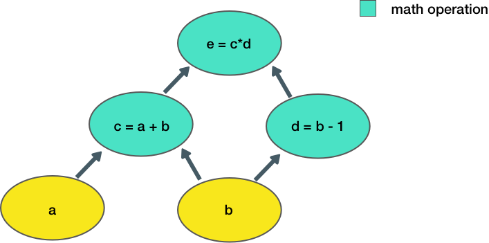
| "Now let's consider a slightly more complicated example:\n", | |
| "\n", | |
| "\n", | |
| "\n", | |
| "Here, we take two inputs, `a, b`, and compute an output `e`. Each node in the graph represents an operation that takes some input, does some computation, and passes its output to another node.\n", | |
| "\n", | |
| "Let's define a simple function in TensorFlow to construct this computation function:" | |
| ] | |
| }, | |
| { | |
| "cell_type": "code", | |
| "metadata": { | |
| "scrolled": true, | |
| "id": "PJnfzpWyYZ23" | |
| }, | |
| "source": [ | |
| "### Defining Tensor computations ###\n", | |
| "\n", | |
| "# Construct a simple computation function\n", | |
| "def func(a,b):\n", | |
| " '''TODO: Define the operation for c, d, e (use tf.add, tf.subtract, tf.multiply).'''\n", | |
| " c = tf.add(a, b)\n", | |
| " d = tf.subtract(b, 1)\n", | |
| " e = tf.multiply(c, d)\n", | |
| " return e" | |
| ], | |
| "execution_count": 9, | |
| "outputs": [] | |
| }, | |
| { | |
| "cell_type": "markdown", | |
| "metadata": { | |
| "id": "AwrRfDMS2-oy" | |
| }, | |
| "source": [ | |
| "Now, we can call this function to execute the computation graph given some inputs `a,b`:" | |
| ] | |
| }, | |
| { | |
| "cell_type": "code", | |
| "metadata": { | |
| "id": "pnwsf8w2uF7p", | |
| "outputId": "1ba0101f-00a6-4375-a198-b1fe97d121bd", | |
| "colab": { | |
| "base_uri": "https://localhost:8080/" | |
| } | |
| }, | |
| "source": [ | |
| "# Consider example values for a,b\n", | |
| "a, b = 1.5, 2.5\n", | |
| "# Execute the computation\n", | |
| "e_out = func(a,b)\n", | |
| "print(e_out)" | |
| ], | |
| "execution_count": 10, | |
| "outputs": [ | |
| { | |
| "output_type": "stream", | |
| "text": [ | |
| "tf.Tensor(6.0, shape=(), dtype=float32)\n" | |
| ], | |
| "name": "stdout" | |
| } | |
| ] | |
| }, | |
| { | |
| "cell_type": "markdown", | |
| "metadata": { | |
| "id": "6HqgUIUhYZ29" | |
| }, | |
| "source": [ | |
| "Notice how our output is a Tensor with value defined by the output of the computation, and that the output has no shape as it is a single scalar value." | |
| ] | |
| }, | |
| { | |
| "cell_type": "markdown", | |
| "metadata": { | |
| "id": "1h4o9Bb0YZ29" | |
| }, | |
| "source": [ | |
| "## 1.3 Neural networks in TensorFlow\n", | |
| "We can also define neural networks in TensorFlow. TensorFlow uses a high-level API called [Keras](https://www.tensorflow.org/guide/keras) that provides a powerful, intuitive framework for building and training deep learning models.\n", | |
| "\n", | |
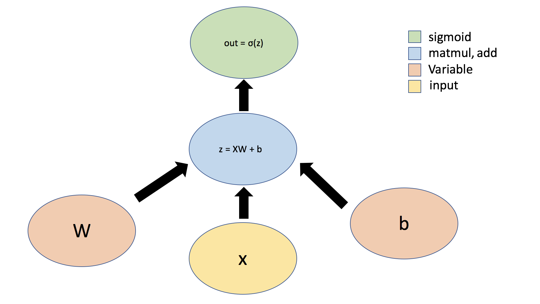
| "Let's first consider the example of a simple perceptron defined by just one dense layer: $ y = \\sigma(Wx + b)$, where $W$ represents a matrix of weights, $b$ is a bias, $x$ is the input, $\\sigma$ is the sigmoid activation function, and $y$ is the output. We can also visualize this operation using a graph: \n", | |
| "\n", | |
| "\n", | |
| "\n", | |
| "Tensors can flow through abstract types called [```Layers```](https://www.tensorflow.org/api_docs/python/tf/keras/layers/Layer) -- the building blocks of neural networks. ```Layers``` implement common neural networks operations, and are used to update weights, compute losses, and define inter-layer connectivity. We will first define a ```Layer``` to implement the simple perceptron defined above." | |
| ] | |
| }, | |
| { | |
| "cell_type": "code", | |
| "metadata": { | |
| "id": "HutbJk-1kHPh", | |
| "outputId": "9f3298c4-4ae4-46a5-ba59-0556ce529ef3", | |
| "colab": { | |
| "base_uri": "https://localhost:8080/" | |
| } | |
| }, | |
| "source": [ | |
| "### Defining a network Layer ###\n", | |
| "\n", | |
| "# n_output_nodes: number of output nodes\n", | |
| "# input_shape: shape of the input\n", | |
| "# x: input to the layer\n", | |
| "\n", | |
| "class OurDenseLayer(tf.keras.layers.Layer):\n", | |
| " def __init__(self, n_output_nodes):\n", | |
| " super(OurDenseLayer, self).__init__()\n", | |
| " self.n_output_nodes = n_output_nodes\n", | |
| "\n", | |
| " def build(self, input_shape):\n", | |
| " d = int(input_shape[-1])\n", | |
| " # Define and initialize parameters: a weight matrix W and bias b\n", | |
| " # Note that parameter initialization is random!\n", | |
| " self.W = self.add_weight(\"weight\", shape=[d, self.n_output_nodes]) # note the dimensionality\n", | |
| " self.b = self.add_weight(\"bias\", shape=[1, self.n_output_nodes]) # note the dimensionality\n", | |
| "\n", | |
| " def call(self, x):\n", | |
| " '''TODO: define the operation for z (hint: use tf.matmul)'''\n", | |
| " z = tf.add(tf.matmul(x, self.W), self.b)\n", | |
| "\n", | |
| " '''TODO: define the operation for out (hint: use tf.sigmoid)'''\n", | |
| " y = tf.sigmoid(z)\n", | |
| " return y\n", | |
| "\n", | |
| "# Since layer parameters are initialized randomly, we will set a random seed for reproducibility\n", | |
| "tf.random.set_seed(1)\n", | |
| "layer = OurDenseLayer(3)\n", | |
| "layer.build((1,2))\n", | |
| "x_input = tf.constant([[1,2.]], shape=(1,2))\n", | |
| "y = layer.call(x_input)\n", | |
| "\n", | |
| "# test the output!\n", | |
| "print(y.numpy())\n", | |
| "mdl.lab1.test_custom_dense_layer_output(y)" | |
| ], | |
| "execution_count": 11, | |
| "outputs": [ | |
| { | |
| "output_type": "stream", | |
| "text": [ | |
| "[[0.2697859 0.45750412 0.66536945]]\n", | |
| "[PASS] test_custom_dense_layer_output\n" | |
| ], | |
| "name": "stdout" | |
| }, | |
| { | |
| "output_type": "execute_result", | |
| "data": { | |
| "text/plain": [ | |
| "True" | |
| ] | |
| }, | |
| "metadata": { | |
| "tags": [] | |
| }, | |
| "execution_count": 11 | |
| } | |
| ] | |
| }, | |
| { | |
| "cell_type": "markdown", | |
| "metadata": { | |
| "id": "Jt1FgM7qYZ3D" | |
| }, | |
| "source": [ | |
| "Conveniently, TensorFlow has defined a number of ```Layers``` that are commonly used in neural networks, for example a [```Dense```](https://www.tensorflow.org/api_docs/python/tf/keras/layers/Dense?version=stable). Now, instead of using a single ```Layer``` to define our simple neural network, we'll use the [`Sequential`](https://www.tensorflow.org/versions/r2.0/api_docs/python/tf/keras/Sequential) model from Keras and a single [`Dense` ](https://www.tensorflow.org/versions/r2.0/api_docs/python/tf/keras/layers/Dense) layer to define our network. With the `Sequential` API, you can readily create neural networks by stacking together layers like building blocks. " | |
| ] | |
| }, | |
| { | |
| "cell_type": "code", | |
| "metadata": { | |
| "id": "7WXTpmoL6TDz" | |
| }, | |
| "source": [ | |
| "### Defining a neural network using the Sequential API ###\n", | |
| "\n", | |
| "# Import relevant packages\n", | |
| "from tensorflow.keras import Sequential\n", | |
| "from tensorflow.keras.layers import Dense\n", | |
| "\n", | |
| "# Define the number of outputs\n", | |
| "n_output_nodes = 3\n", | |
| "\n", | |
| "# First define the model \n", | |
| "model = Sequential()\n", | |
| "\n", | |
| "'''TODO: Define a dense (fully connected) layer to compute z'''\n", | |
| "# Remember: dense layers are defined by the parameters W and b!\n", | |
| "# You can read more about the initialization of W and b in the TF documentation :) \n", | |
| "# https://www.tensorflow.org/api_docs/python/tf/keras/layers/Dense?version=stable\n", | |
| "dense_layer = Dense(units=2)\n", | |
| "\n", | |
| "# Add the dense layer to the model\n", | |
| "model.add(dense_layer)\n" | |
| ], | |
| "execution_count": 12, | |
| "outputs": [] | |
| }, | |
| { | |
| "cell_type": "markdown", | |
| "metadata": { | |
| "id": "HDGcwYfUyR-U" | |
| }, | |
| "source": [ | |
| "That's it! We've defined our model using the Sequential API. Now, we can test it out using an example input:" | |
| ] | |
| }, | |
| { | |
| "cell_type": "code", | |
| "metadata": { | |
| "id": "sg23OczByRDb", | |
| "outputId": "0baaced8-1e46-480d-c4fe-22ec06642b16", | |
| "colab": { | |
| "base_uri": "https://localhost:8080/" | |
| } | |
| }, | |
| "source": [ | |
| "# Test model with example input\n", | |
| "x_input = tf.constant([[1,2.]], shape=(1,2))\n", | |
| "\n", | |
| "'''TODO: feed input into the model and predict the output!'''\n", | |
| "model_output = model(x_input)\n", | |
| "print(model_output)" | |
| ], | |
| "execution_count": 14, | |
| "outputs": [ | |
| { | |
| "output_type": "stream", | |
| "text": [ | |
| "tf.Tensor([[ 0.8787118 -0.20480263]], shape=(1, 2), dtype=float32)\n" | |
| ], | |
| "name": "stdout" | |
| } | |
| ] | |
| }, | |
| { | |
| "cell_type": "markdown", | |
| "metadata": { | |
| "id": "596NvsOOtr9F" | |
| }, | |
| "source": [ | |
| "In addition to defining models using the `Sequential` API, we can also define neural networks by directly subclassing the [`Model`](https://www.tensorflow.org/api_docs/python/tf/keras/Model?version=stable) class, which groups layers together to enable model training and inference. The `Model` class captures what we refer to as a \"model\" or as a \"network\". Using Subclassing, we can create a class for our model, and then define the forward pass through the network using the `call` function. Subclassing affords the flexibility to define custom layers, custom training loops, custom activation functions, and custom models. Let's define the same neural network as above now using Subclassing rather than the `Sequential` model." | |
| ] | |
| }, | |
| { | |
| "cell_type": "code", | |
| "metadata": { | |
| "id": "K4aCflPVyViD" | |
| }, | |
| "source": [ | |
| "### Defining a model using subclassing ###\n", | |
| "\n", | |
| "from tensorflow.keras import Model\n", | |
| "from tensorflow.keras.layers import Dense\n", | |
| "\n", | |
| "class SubclassModel(tf.keras.Model):\n", | |
| "\n", | |
| " # In __init__, we define the Model's layers\n", | |
| " def __init__(self, n_output_nodes):\n", | |
| " super(SubclassModel, self).__init__()\n", | |
| " '''TODO: Our model consists of a single Dense layer. Define this layer.''' \n", | |
| " self.dense_layer = Dense(units=2)\n", | |
| "\n", | |
| " # In the call function, we define the Model's forward pass.\n", | |
| " def call(self, inputs):\n", | |
| " return self.dense_layer(inputs)" | |
| ], | |
| "execution_count": 15, | |
| "outputs": [] | |
| }, | |
| { | |
| "cell_type": "markdown", | |
| "metadata": { | |
| "id": "U0-lwHDk4irB" | |
| }, | |
| "source": [ | |
| "Just like the model we built using the `Sequential` API, let's test out our `SubclassModel` using an example input.\n", | |
| "\n" | |
| ] | |
| }, | |
| { | |
| "cell_type": "code", | |
| "metadata": { | |
| "id": "LhB34RA-4gXb", | |
| "outputId": "8de724fa-0a74-4a88-8e12-d7f29d68b68d", | |
| "colab": { | |
| "base_uri": "https://localhost:8080/" | |
| } | |
| }, | |
| "source": [ | |
| "n_output_nodes = 3\n", | |
| "model = SubclassModel(n_output_nodes)\n", | |
| "\n", | |
| "x_input = tf.constant([[1,2.]], shape=(1,2))\n", | |
| "\n", | |
| "print(model.call(x_input))" | |
| ], | |
| "execution_count": 16, | |
| "outputs": [ | |
| { | |
| "output_type": "stream", | |
| "text": [ | |
| "tf.Tensor([[-0.6277685 0.7001949]], shape=(1, 2), dtype=float32)\n" | |
| ], | |
| "name": "stdout" | |
| } | |
| ] | |
| }, | |
| { | |
| "cell_type": "markdown", | |
| "metadata": { | |
| "id": "HTIFMJLAzsyE" | |
| }, | |
| "source": [ | |
| "Importantly, Subclassing affords us a lot of flexibility to define custom models. For example, we can use boolean arguments in the `call` function to specify different network behaviors, for example different behaviors during training and inference. Let's suppose under some instances we want our network to simply output the input, without any perturbation. We define a boolean argument `isidentity` to control this behavior:" | |
| ] | |
| }, | |
| { | |
| "cell_type": "code", | |
| "metadata": { | |
| "id": "P7jzGX5D1xT5" | |
| }, | |
| "source": [ | |
| "### Defining a model using subclassing and specifying custom behavior ###\n", | |
| "\n", | |
| "from tensorflow.keras import Model\n", | |
| "from tensorflow.keras.layers import Dense\n", | |
| "\n", | |
| "class IdentityModel(tf.keras.Model):\n", | |
| "\n", | |
| " # As before, in __init__ we define the Model's layers\n", | |
| " # Since our desired behavior involves the forward pass, this part is unchanged\n", | |
| " def __init__(self, n_output_nodes):\n", | |
| " super(IdentityModel, self).__init__()\n", | |
| " self.dense_layer = tf.keras.layers.Dense(n_output_nodes, activation='sigmoid')\n", | |
| "\n", | |
| " '''TODO: Implement the behavior where the network outputs the input, unchanged, \n", | |
| " under control of the isidentity argument.'''\n", | |
| " def call(self, inputs, isidentity=False):\n", | |
| " x = self.dense_layer(inputs)\n", | |
| " if isidentity:\n", | |
| " return inputs\n", | |
| " else:\n", | |
| " return self.dense_layer(inputs)" | |
| ], | |
| "execution_count": 20, | |
| "outputs": [] | |
| }, | |
| { | |
| "cell_type": "markdown", | |
| "metadata": { | |
| "id": "Ku4rcCGx5T3y" | |
| }, | |
| "source": [ | |
| "Let's test this behavior:" | |
| ] | |
| }, | |
| { | |
| "cell_type": "code", | |
| "metadata": { | |
| "id": "NzC0mgbk5dp2", | |
| "outputId": "188603c2-566d-46b5-e7a0-4ece283182ec", | |
| "colab": { | |
| "base_uri": "https://localhost:8080/" | |
| } | |
| }, | |
| "source": [ | |
| "n_output_nodes = 3\n", | |
| "model = IdentityModel(n_output_nodes)\n", | |
| "\n", | |
| "x_input = tf.constant([[1,2.]], shape=(1,2))\n", | |
| "'''TODO: pass the input into the model and call with and without the input identity option.'''\n", | |
| "out_activate = model.call(x_input)\n", | |
| "out_identity = model.call(x_input, isidentity=True)\n", | |
| "\n", | |
| "print(\"Network output with activation: {}; network identity output: {}\".format(out_activate.numpy(), out_identity.numpy()))" | |
| ], | |
| "execution_count": 21, | |
| "outputs": [ | |
| { | |
| "output_type": "stream", | |
| "text": [ | |
| "Network output with activation: [[0.19695838 0.6330006 0.7668015 ]]; network identity output: [[1. 2.]]\n" | |
| ], | |
| "name": "stdout" | |
| } | |
| ] | |
| }, | |
| { | |
| "cell_type": "markdown", | |
| "metadata": { | |
| "id": "7V1dEqdk6VI5" | |
| }, | |
| "source": [ | |
| "Now that we have learned how to define `Layers` as well as neural networks in TensorFlow using both the `Sequential` and Subclassing APIs, we're ready to turn our attention to how to actually implement network training with backpropagation." | |
| ] | |
| }, | |
| { | |
| "cell_type": "markdown", | |
| "metadata": { | |
| "id": "dQwDhKn8kbO2" | |
| }, | |
| "source": [ | |
| "## 1.4 Automatic differentiation in TensorFlow\n", | |
| "\n", | |
| "[Automatic differentiation](https://en.wikipedia.org/wiki/Automatic_differentiation)\n", | |
| "is one of the most important parts of TensorFlow and is the backbone of training with \n", | |
| "[backpropagation](https://en.wikipedia.org/wiki/Backpropagation). We will use the TensorFlow GradientTape [`tf.GradientTape`](https://www.tensorflow.org/api_docs/python/tf/GradientTape?version=stable) to trace operations for computing gradients later. \n", | |
| "\n", | |
| "When a forward pass is made through the network, all forward-pass operations get recorded to a \"tape\"; then, to compute the gradient, the tape is played backwards. By default, the tape is discarded after it is played backwards; this means that a particular `tf.GradientTape` can only\n", | |
| "compute one gradient, and subsequent calls throw a runtime error. However, we can compute multiple gradients over the same computation by creating a ```persistent``` gradient tape. \n", | |
| "\n", | |
| "First, we will look at how we can compute gradients using GradientTape and access them for computation. We define the simple function $ y = x^2$ and compute the gradient:" | |
| ] | |
| }, | |
| { | |
| "cell_type": "code", | |
| "metadata": { | |
| "id": "tdkqk8pw5yJM" | |
| }, | |
| "source": [ | |
| "### Gradient computation with GradientTape ###\n", | |
| "\n", | |
| "# y = x^2\n", | |
| "# Example: x = 3.0\n", | |
| "x = tf.Variable(3.0)\n", | |
| "\n", | |
| "# Initiate the gradient tape\n", | |
| "with tf.GradientTape() as tape:\n", | |
| " # Define the function\n", | |
| " y = x * x\n", | |
| "# Access the gradient -- derivative of y with respect to x\n", | |
| "dy_dx = tape.gradient(y, x)\n", | |
| "\n", | |
| "assert dy_dx.numpy() == 6.0" | |
| ], | |
| "execution_count": 22, | |
| "outputs": [] | |
| }, | |
| { | |
| "cell_type": "markdown", | |
| "metadata": { | |
| "id": "JhU5metS5xF3" | |
| }, | |
| "source": [ | |
| "In training neural networks, we use differentiation and stochastic gradient descent (SGD) to optimize a loss function. Now that we have a sense of how `GradientTape` can be used to compute and access derivatives, we will look at an example where we use automatic differentiation and SGD to find the minimum of $L=(x-x_f)^2$. Here $x_f$ is a variable for a desired value we are trying to optimize for; $L$ represents a loss that we are trying to minimize. While we can clearly solve this problem analytically ($x_{min}=x_f$), considering how we can compute this using `GradientTape` sets us up nicely for future labs where we use gradient descent to optimize entire neural network losses." | |
| ] | |
| }, | |
| { | |
| "cell_type": "code", | |
| "metadata": { | |
| "attributes": { | |
| "classes": [ | |
| "py" | |
| ], | |
| "id": "" | |
| }, | |
| "id": "7g1yWiSXqEf-", | |
| "outputId": "9eae6abb-532c-4139-fba3-43461b93bc4e", | |
| "colab": { | |
| "base_uri": "https://localhost:8080/", | |
| "height": 313 | |
| } | |
| }, | |
| "source": [ | |
| "### Function minimization with automatic differentiation and SGD ###\n", | |
| "\n", | |
| "# Initialize a random value for our initial x\n", | |
| "x = tf.Variable([tf.random.normal([1])])\n", | |
| "print(\"Initializing x={}\".format(x.numpy()))\n", | |
| "\n", | |
| "learning_rate = 1e-2 # learning rate for SGD\n", | |
| "history = []\n", | |
| "# Define the target value\n", | |
| "x_f = 4\n", | |
| "\n", | |
| "# We will run SGD for a number of iterations. At each iteration, we compute the loss, \n", | |
| "# compute the derivative of the loss with respect to x, and perform the SGD update.\n", | |
| "for i in range(500):\n", | |
| " with tf.GradientTape() as tape:\n", | |
| " '''TODO: define the loss as described above'''\n", | |
| " loss = tf.square(x - x_f)\n", | |
| "\n", | |
| " # loss minimization using gradient tape\n", | |
| " grad = tape.gradient(loss, x) # compute the derivative of the loss with respect to x\n", | |
| " new_x = x - learning_rate*grad # sgd update\n", | |
| " x.assign(new_x) # update the value of x\n", | |
| " history.append(x.numpy()[0])\n", | |
| "\n", | |
| "# Plot the evolution of x as we optimize towards x_f!\n", | |
| "plt.plot(history)\n", | |
| "plt.plot([0, 500],[x_f,x_f])\n", | |
| "plt.legend(('Predicted', 'True'))\n", | |
| "plt.xlabel('Iteration')\n", | |
| "plt.ylabel('x value')" | |
| ], | |
| "execution_count": 23, | |
| "outputs": [ | |
| { | |
| "output_type": "stream", | |
| "text": [ | |
| "Initializing x=[[-0.00839665]]\n" | |
| ], | |
| "name": "stdout" | |
| }, | |
| { | |
| "output_type": "execute_result", | |
| "data": { | |
| "text/plain": [ | |
| "Text(0, 0.5, 'x value')" | |
| ] | |
| }, | |
| "metadata": { | |
| "tags": [] | |
| }, | |
| "execution_count": 23 | |
| }, | |
| { | |
| "output_type": "display_data", | |
| "data": { | |
| "image/png": "iVBORw0KGgoAAAANSUhEUgAAAYIAAAEGCAYAAABo25JHAAAABHNCSVQICAgIfAhkiAAAAAlwSFlzAAALEgAACxIB0t1+/AAAADh0RVh0U29mdHdhcmUAbWF0cGxvdGxpYiB2ZXJzaW9uMy4yLjIsIGh0dHA6Ly9tYXRwbG90bGliLm9yZy+WH4yJAAAgAElEQVR4nO3deXxV9Z3/8dcnNwlhX0JEVhMRxIAIGhDrRt1trVardZlWbVW0Yzttp320tr9HXdqZqTPTR9tRO3UY9VGt1tKqbakjrtWiokhYZEkEAgiELSGBLED2z++Pe8AQEwmQk5N77/v58D7uWb735PON4Xzu+X7P+X7N3RERkdSVFnUAIiISLSUCEZEUp0QgIpLilAhERFKcEoGISIpLjzqAwzV06FDPzc2NOgwRkYSyePHine6e096+hEsEubm5FBYWRh2GiEhCMbONHe1T05CISIpTIhARSXFKBCIiKU6JQEQkxSkRiIikuNATgZnFzGypmT3fzr5eZjbHzErMbKGZ5YYdj4iIHKw7rgi+CRR3sO8WYJe7nwD8Avj3bohHRERaCfU5AjMbBXwW+Ffgn9spcgVwb7D8DPCQmZmHMTb2vLtg+4ouP6xIlBzHHRxw9+A9vj34L17OPyrf4faD1gnKtbfdP/o8bRfaXQ2O0f4/649t9fY//1E07f+A9n9muwc6Ah8/0GEf+jA+0F7RWJox4sTpcOn9h/uTDynsB8p+CXwP6N/B/pHAZgB3bzKzKiAb2Nm6kJnNAmYBjBkzJrRgRTpr/wm4ucVpdqcleG9ucVpaoMU9eMVPgC3+Cdta4sdqOXAiP/jk3uIfnYBb+OhEr6lEUkt6mjEirGOHdFzM7DKgzN0Xm9nMozmWu88GZgMUFBQc2Z9/CFlUEtu+hmYq9zawe28DVXsbqdrXyO59jewOlqv2NcS37W2ktr6JPfVN7KlvZk9DE3sbmmluObw/RTPolZ5Gr/QYWRnx914ZafFXeozMWBrpMSMjlkZ6mpEeM9LTgm3Be3z7R9tiaUZGLNiW9tH+WJoRM8MM0syIpR28nGZgFi+TltZq2eL70tI6WA7K7D+eBfUCC973b7NW+8Ba7z/w/lGZ+BIHjom1+UwHx8RafeYTjtnR/492t9P+jvbKd3AIrIODt7e14/g6OnrXC/OK4EzgcjP7DJAFDDCzJ939S63KbAFGA6Vmlg4MBCpCjElSQHVdI1t372Pr7n2UVddTXlPPztp6ymv3LzdQXlNPbX1Th8fIjKUxoHcGg/pkMLB3BkP6ZjJ6cB/6ZMbo2yudvr2C98x0+mTG6NcrnT690umbGaNPZnr8RJ8RC0788RN9Rsy69R+3SGeFlgjc/QfADwCCK4LvtkkCAHOBm4B3gKuBv4XSPyBJpaGphU2Ve1hXvoeNFXvYsmsfW3bvozR4r6n7+Al+QFY6Of17kdO/F5NGDmRov0xy+vciu28mA3tnHjjh73/vnRHTSVtSRrcPOmdmPwYK3X0u8CjwWzMrASqB67o7Hum59jU0s3pHDcXbqllXVsv6nXtYX17L5l37DmqW6d8rnZGDezNyUG+m5w1h5KDejBzcmxGDejNsQBbZfTPJyohFWBORns0S7Qt4QUGBa/TR5FO1r5H3N++maFs1RVurKdpWzfryWvaf73ulp5E3tC9jc/pxfE5fjs/pS97QfuRl92Vgn4xogxdJAGa22N0L2tuXcMNQS+Jzdz6s2MvijbtYvHEXSzbuYk1ZzYG7YEYO6k3+iAF89uTh5I8YQP7wAYwc1Ju0NDXViIRBiUC6RVl1HW+V7OSttTt5q2QnZTX1APTPSufUMYP57OThnHbcYCaNGKhv+CLdTIlAQtHS4rxfupuXVu3g9Q/KWL2jBoDBfTI484ShnDE2m4LjhjDumH76pi8SMSUC6TJNzS0s3FDJiyu383LRdnZU15OeZkzPG8L3p07g7HFDyR8+QCd+kR5GiUCOWvG2ap5bUsqfl22lvKaerIw0zh2fw8UTj+X8CcPU1CPSwykRyBGpqWvk2cWl/KGwlKJt1aSnGedNOIYrp45k5onH0DtTt2uKJAolAjksJWW1PPHOhzy7uJQ9Dc2cPHIg910+kc+dMoIhfTOjDk9EjoASgXTKwvUV/OqNdcxfU05mLI3LJg/npk/lcsroQVGHJiJHSYlAOuTuvLl2Jw/9rYT3PqxkaL9MvnPheK4/fQxD+/WKOjwR6SJKBNKuxRsr+bcXPmDxxl0MH5jFfZdP5NppozVUg0gSUiKQg6wvr+U/XlzNi6u2c0z/XvzrlZO45rTRZKZremuRZKVEIADsqW/iv15by2NvbaBXehrfuXA8t5ydR59M/YmIJDv9KxdeXrWde+euYmtVHdcWjOa7F59ITn/1AYikCiWCFFZeU8//+9MKXi7awYnD+vPM9VMpyB0SdVgi0s2UCFLUK0U7uOvZ5dTUN3HXpRO45aw8MmLqBxBJRUoEKaa2vomf/LWIOYWbyR8+gKevm8L4Yf2jDktEIhTm5PVZwHygV/BznnH3e9qUuRn4T+JzFwM85O6PhBVTqlu7o4bbn1zMhp17+NrMsXz7gvG6G0hEQr0iqAfOc/daM8sA3jKzee7+bptyc9z96yHGIcBf39/K959dTp/MGE/dejqfGjs06pBEpIcIc/J6B2qD1YzglVjzYiaBlhbn/hc/YPb89Zx23GB+dcOpHDswK+qwRKQHCbVdwMxiZrYMKANecfeF7RT7gpktN7NnzGx0B8eZZWaFZlZYXl4eZshJZV9DM//41BJmz1/Pl2aM4enbZigJiMjHhJoI3L3Z3acAo4DpZjapTZG/ArnuPhl4BXi8g+PMdvcCdy/IyckJM+SkUV5Tz3X/+y4vFW3nR5fl85MrJqk/QETa1S1nBnffDbwOXNJme4W71werjwCndUc8ya50116ufngBa7bX8D9fOo1bzsrDTLOCiUj7QksEZpZjZoOC5d7AhcAHbcoMb7V6OVAcVjypYsPOPXzx4XfYtaeBp247nYsmHht1SCLSw4V519Bw4HEzixFPOH9w9+fN7MdAobvPBf7JzC4HmoBK4OYQ40l6q7fX8A+PLKTFnadnzWDiiIFRhyQiCcDiN/ckjoKCAi8sLIw6jB5nXXktX3z4HWJpxu9uO50TjtFDYiLyETNb7O4F7e3Tk8VJYHPlXr70yELM4OlZMxib0y/qkEQkgeg2kgS3o7qOf3hkIXvqm3jiq6crCYjIYVMiSGA1dY3c9Nh7VNTW8/hXp5M/YkDUIYlIAlLTUIJqam7hzt8tpaSslt98ZTpTxwyOOiQRSVBKBAnI3bl77irmrynn/qtO5qxxGjdIRI6cmoYS0KNvbeB3Czdxx7ljuW76mKjDEZEEp0SQYBaU7OTfXijm0knH8r2LT4w6HBFJAkoECWR7VR3feHopx+f042fXnEJamoaNEJGjpz6CBNHQ1MI/PrWYfY3NzPnSqfTtpf91ItI1dDZJEPfP+4Alm3bz0A1T9dSwiHQpNQ0lgNdXl/HY2xu4+VO5XDZ5RNThiEiSUSLo4Sr3NPC9Z5Zz4rD+3HXphKjDEZEkpKahHszduevZ5VTtbeTxr0wnKyMWdUgikoR0RdCD/bGwlJeLdvDdi8dr+AgRCY0SQQ+1rWofP36+iBnHD+HWs46POhwRSWJKBD3UPX9ZRVNLC//xBT0vICLhCnOqyiwze8/M3jezVWZ2XztlepnZHDMrMbOFZpYbVjyJ5MWV23m5aAffumA8Y7L7RB2OiCS5MK8I6oHz3P0UYApwiZnNaFPmFmCXu58A/AL49xDjSQjVdY3cM3clJw0fwC1n5UUdjoikgNASgcfVBqsZwavtvJhXAI8Hy88A55tZSreD/OeLqymvqef+q04mI6aWOxEJX6hnGjOLmdkyoAx4xd0XtikyEtgM4O5NQBWQHWZMPdnKLVU8uXAjN56RyymjB0UdjoikiFATgbs3u/sUYBQw3cwmHclxzGyWmRWaWWF5eXnXBtlDuDs/eb6IwX0y+faF46MOR0RSSLe0Pbj7buB14JI2u7YAowHMLB0YCFS08/nZ7l7g7gU5OTlhhxuJF1duZ+GGSv75wvEM7J0RdTgikkLCvGsox8wGBcu9gQuBD9oUmwvcFCxfDfzN3dv2IyS9usZm/m1eMROO7c9100ZHHY6IpJgwh5gYDjxuZjHiCecP7v68mf0YKHT3ucCjwG/NrASoBK4LMZ4e67G3N7C5ch9P3Xo66eogFpFuFloicPflwNR2tt/darkOuCasGBJBRW09v/pbCRecNIwzT9DcwyLS/fT1M2L/M389+xqbuetSTTspItFQIojQjuo6Hl/wIZ+fOlKTzYhIZJQIIvSr10tobnG+db5uFxWR6CgRRKR0116efm8TX5w2WuMJiUiklAgi8sBrazEzvnHeCVGHIiIpTokgApsr9/Lski3cMH0Mwwf2jjocEUlxSgQR+N8315NmcMe5Y6MORUREiaC77aytZ86izVw1dRTHDsyKOhwRESWC7vabtz+kobmFWedq+kkR6RmUCLpRbX0TT7zzIRfnH8vYnH5RhyMiAigRdKunF26iuq6JO2aqb0BEeg4lgm7S0NTCI2+t51Njs5miSWdEpAdRIugm81ZuY0d1Pbedo74BEelZlAi6yRPvbCQ3uw/njkvOiXVEJHEpEXSDlVuqWLxxF18+I5e0NIs6HBGRgygRdIPHF3xIn8wYV582KupQREQ+RokgZLv2NPCX97dy5dSRmotYRHqkMOcsHm1mr5tZkZmtMrNvtlNmpplVmdmy4HV3e8dKZHMKN9PQ1MKNZ+RGHYqISLvCnLO4CfiOuy8xs/7AYjN7xd2L2pR7090vCzGOyDS3OL99ZyMzjh/Cicdq4hkR6ZlCuyJw923uviRYrgGKgZFh/byeaP7acrbs3qerARHp0bqlj8DMcolPZL+wnd1nmNn7ZjbPzCZ28PlZZlZoZoXl5eUhRtq1/rBoM9l9M7ngpGFRhyIi0qHQE4GZ9QOeBb7l7tVtdi8BjnP3U4AHgT+3dwx3n+3uBe5ekJOTGPfhV9TW82rxDq6cOpLMdPXJi0jPFeoZyswyiCeBp9z9ubb73b3a3WuD5ReADDMbGmZM3eVPS7fQ2Ox8cdroqEMREflEYd41ZMCjQLG7/7yDMscG5TCz6UE8FWHF1F3cnTmLNjNl9CDGD1MnsYj0bGHeNXQm8GVghZktC7b9EBgD4O4PA1cDXzOzJmAfcJ27e4gxdYtlm3eztqyWn151ctShiIgcUmiJwN3fAj5xPAV3fwh4KKwYovLHxaX0zohx2eThUYciInJI6sXsYg1NLbywYhsXTRxG/yw9SSwiPd8hE4GZDTOzR81sXrCeb2a3hB9aYvr7mnJ2723k81NS6pEJEUlgnbki+A3wEjAiWF8DfCusgBLdn5dtYUjfTM4alxQ3P4lICuhMIhjq7n8AWgDcvQloDjWqBFVT18irRTu4bPJwMmJqdRORxNCZs9UeM8sGHMDMZgBVoUaVoF5cuZ36phY+P1XNQiKSODpz19A/A3OBsWb2NpBD/LZPaeMvy7ZyXHYfpmpOYhFJIIdMBMHooecCJxK/HXS1uzeGHlmC2Vlbz4J1O7nz0ycQPCMnIpIQDpkIzOzGNptONTPc/YmQYkpIL63aTovDZ/XsgIgkmM40DU1rtZwFnE98sDglglbmrdjO8UP7cqKGlBCRBNOZpqFvtF43s0HA70OLKAFV7mngnfUV3HHu8WoWEpGEcyT3OO4B8ro6kET2StF2mlucSyepWUhEEk9n+gj+SnDrKPHEkQ/8IcygEs0LK7YzZkgfJo4YEHUoIiKHrTN9BD9rtdwEbHT30pDiSThVext5u2Qnt5ydp2YhEUlInekj+Ht3BJKoXineQZOahUQkgXWYCMysho+ahA7aBbi7qx2EeP/AsQOyOGXUwKhDERE5Ih0mAnfXfZCHUNfYzJtrd3Ll1JFqFhKRhNXpu4bM7BgzG7P/1Ynyo83sdTMrMrNVZvbNdsqYmT1gZiVmttzMTj3cCkTpnfUV7G1o5oL8YVGHIiJyxDozH8HlZrYW2AD8HfgQmNeJYzcB33H3fGAGcKeZ5bcpcykwLnjNAn7d+dCj91rxDvpkxjjj+OyoQxEROWKduSL4CfET+Rp3zyP+ZPG7h/qQu29z9yXBcg1QDLQdlvMK4AmPexcYZGYJ0evq7rxaVMbZ44aSlRGLOhwRkSPWmUTQ6O4VQJqZpbn760DB4fwQM8sFpgIL2+waCWxutV7Kx5MFZjbLzArNrLC8vPxwfnRoVm2tZnt1HRecpGYhEUlsnXmOYLeZ9QPmA0+ZWRnxp4s7Jfjss8C33L36SIJ099nAbICCgoL27mTqdq8W78AMPj3hmKhDERE5Kp25IrgC2At8G3gRWAd8rjMHN7MM4kngKXd/rp0iW4DRrdZHBdt6vNeKyzh1zGCG9usVdSgiIkelM4ngdmC4uze5++Pu/kDQVPSJLH4/5aNAsbv/vINic4Ebg7uHZgBV7r6t09FHpLymnhVbqvj0iTlRhyIictQ60zTUH3jZzCqBOcAf3X1HJz53JvBlYIWZLQu2/RAYA+DuDwMvAJ8BSohfdXzl8MKPxlsl8X6Kc8erWUhEEl9nhpi4D7jPzCYD1wJ/N7NSd7/gEJ97i/hTyJ9UxoE7DyPeHuHvq8vJ7pupQeZEJCkczjDUZcB2oAJI2a/CLS3Om2t3cva4oaSl6WliEUl8nXmg7B/N7A3gNSAbuM3dJ4cdWE+1ams1FXsaOGe8+gdEJDl0po9gNPFbP5cdsmQKmL823j9w9jglAhFJDp3pI/hBdwSSKP6+ppyJIwaQ01+3jYpIcjiSqSpTVk1dI0s27uJcNQuJSBJRIjgM76yroKnF1T8gIkmlM53FbUcMxcxmhhJND7dgXQVZGWmcOmZw1KGIiHSZzlwR/MHMvh88/dvbzB4Efhp2YD3RO+sqmJY7hMx0XUiJSPLozBntdOJ3Di0AFgFbiT81nFLKa+pZvaOGT40dGnUoIiJdqlPDUAP7gN5AFrDB3VtCjaoHend9fHilT43VJDQiklw6kwgWEU8E04CzgevN7I+hRtUDLVhXQf+sdA0rISJJpzMPlN3i7oXB8jbgCjP7cogx9UjvrNvJ6XnZpMfUPyAiyeWQZ7VWSaD1tt+GE07PtGX3Pj6s2KtmIRFJSvp62wnvrAv6B05QIhCR5KNE0AkL1u0ku28m44/pH3UoIiJdTomgE97bUMn0vCEadlpEklJoicDMHjOzMjNb2cH+mWZWZWbLgtfdYcVyNLZV7aN01z6m5Q6JOhQRkVB05q6hI/Ub4CHgiU8o86a7XxZiDEftvQ2VAEzPUyIQkeQU2hWBu88HKsM6fndZ9GEl/Xqlc9JwPT8gIskp6j6CM8zsfTObZ2YTOypkZrPMrNDMCsvLy7szPhZt2MWpxw0mpv4BEUlSUSaCJcBx7n4K8CDw544Kuvtsdy9w94KcnO4bAnr33gZW76hh2nEabVREkldkicDdq929Nlh+Acgwsx41otvijbsAmKb+ARFJYpElAjM71swsWJ4exFIRVTztee/DSjJixpTRg6IORUQkNKHdNWRmTwMzgaFmVgrcA2QAuPvDwNXA18ysifigdte5u4cVz5FYtKGSyaMGkZURizoUEZHQhJYI3P36Q+x/iPjtpT1SXWMzK7ZUcctZx0cdiohIqKK+a6jHWl5aRWOzU6COYhFJckoEHVi6Kd5RPHWM+gdEJLkpEXRg6abd5Gb3Ibtfr6hDEREJlRJBO9ydJZt2MXWMmoVEJPkpEbRja1UdZTX1ahYSkZSgRNCOA/0Do3VFICLJT4mgHUs37aZXehoThmsiGhFJfkoE7Vi6aReTRw0kQxPVi0gK0JmujfqmZlZurVZHsYikDCWCNoq31dDQ1MKp6igWkRShRNDGRw+S6YpARFKDEkEbyzbvZvjALIYNyIo6FBGRbqFE0MaK0ipOHjkw6jBERLqNEkEr1XWNrN+5h8mjlAhEJHUoEbSyaks1ACePUkexiKQOJYJWVmzZDaCmIRFJKaElAjN7zMzKzGxlB/vNzB4wsxIzW25mp4YVS2ctL61i5KDeDOmbGXUoIiLdJswrgt8Al3zC/kuBccFrFvDrEGPplBVbqtQ/ICIpJ7RE4O7zgcpPKHIF8ITHvQsMMrPhYcVzKFV7G9lYsZeTlQhEJMVE2UcwEtjcar002PYxZjbLzArNrLC8vDyUYFZurQLUPyAiqSchOovdfba7F7h7QU5OTig/Y3mpEoGIpKYoE8EWYHSr9VHBtkis2LKbMUP6MKiPOopFJLVEmQjmAjcGdw/NAKrcfVtUwazYoieKRSQ1pYd1YDN7GpgJDDWzUuAeIAPA3R8GXgA+A5QAe4GvhBXLoeze28Dmyn3cMP24qEIQEYlMaInA3a8/xH4H7gzr5x+Oom3xJ4onjhgQcSQiIt0vITqLw1a0NZ4IThquRCAiqUeJgPhkNDn9e5HTv1fUoYiIdDslAuJNQ/m6GhCRFJXyiaChqYWSshry1T8gIikq5RPB2rIaGptdVwQikrJSPhEUb6sB0BWBiKSslE8ERVurycpIIze7b9ShiIhEQolgWxUTjh1ALM2iDkVEJBIpnQjcnaKt1WoWEpGUltKJYGtVHdV1TeooFpGUltKJQE8Ui4ikeCIoDsYYmnBs/4gjERGJTkongtU7ahgzpA99e4U29p6ISI+X0mfANdtrOFFXAyI9QmNjI6WlpdTV1UUdSkLLyspi1KhRZGRkdPozKZsI6pua2bBzDxdPPDbqUEQEKC0tpX///uTm5mKm27mPhLtTUVFBaWkpeXl5nf5cyjYNbdi5h6YWZ7yuCER6hLq6OrKzs5UEjoKZkZ2dfdhXVaEmAjO7xMxWm1mJmd3Vzv6bzazczJYFr1vDjKe11dvjQ0ucOEyJQKSnUBI4ekfyOwxzqsoY8CvgQqAUWGRmc929qE3ROe7+9bDi6MiaHTWkpxl5QzW0hIiktjCvCKYDJe6+3t0bgN8DV4T48w7L6u21HJ/Tl8z0lG0dE5E2YrEYU6ZMYdKkSVxzzTXs3bv3iI91880388wzzwBw6623UlTU9jvwR9544w0WLFhw2D8jNzeXnTt3HnGM+4V5FhwJbG61Xhpsa+sLZrbczJ4xs9HtHcjMZplZoZkVlpeXd0lwa3bUMF7NQiLSSu/evVm2bBkrV64kMzOThx9++KD9TU1NR3TcRx55hPz8/A73H2ki6CpR3zX0V+Bpd683s9uBx4Hz2hZy99nAbICCggI/2h+6t6GJTZV7uea0UUd7KBEJwX1/XXXgyf+ukj9iAPd8bmKny5999tksX76cN954gx/96EcMHjyYDz74gOLiYu666y7eeOMN6uvrufPOO7n99ttxd77xjW/wyiuvMHr0aDIzMw8ca+bMmfzsZz+joKCAF198kR/+8Ic0NzczdOhQHn30UR5++GFisRhPPvkkDz74IBMmTOCOO+5g06ZNAPzyl7/kzDPPpKKiguuvv54tW7Zwxhln4H7Up0Mg3ESwBWj9DX9UsO0Ad69otfoI8B8hxnPAmh21ALpjSETa1dTUxLx587jkkksAWLJkCStXriQvL4/Zs2czcOBAFi1aRH19PWeeeSYXXXQRS5cuZfXq1RQVFbFjxw7y8/P56le/etBxy8vLue2225g/fz55eXlUVlYyZMgQ7rjjDvr168d3v/tdAG644Qa+/e1vc9ZZZ7Fp0yYuvvhiiouLue+++zjrrLO4++67+b//+z8effTRLqlvmIlgETDOzPKIJ4DrgBtaFzCz4e6+LVi9HCgOMZ4D1uiOIZEe7XC+uXelffv2MWXKFCB+RXDLLbewYMECpk+ffuC+/Jdffpnly5cfaP+vqqpi7dq1zJ8/n+uvv55YLMaIESM477yPNW7w7rvvcs455xw41pAhQ9qN49VXXz2oT6G6upra2lrmz5/Pc889B8BnP/tZBg8e3CX1Di0RuHuTmX0deAmIAY+5+yoz+zFQ6O5zgX8ys8uBJqASuDmseFpbvaOGrIw0Rg/p0x0/TkQSxP4+grb69v3o7kJ358EHH+Tiiy8+qMwLL7zQZXG0tLTw7rvvkpWV1WXH/CSh3jLj7i+4+3h3H+vu/xpsuztIArj7D9x9oruf4u6fdvcPwoxnvzU7ahh3TH9NRiMih+3iiy/m17/+NY2NjQCsWbOGPXv2cM455zBnzhyam5vZtm0br7/++sc+O2PGDObPn8+GDRsAqKysBKB///7U1NQcKHfRRRfx4IMPHljfn5zOOeccfve73wEwb948du3a1SV1Ssl7J1dvr2HcsH5RhyEiCejWW28lPz+fU089lUmTJnH77bfT1NTElVdeybhx48jPz+fGG2/kjDPO+Nhnc3JymD17NldddRWnnHIK1157LQCf+9zn+NOf/sSUKVN48803eeCBBygsLGTy5Mnk5+cfuHvpnnvuYf78+UycOJHnnnuOMWPGdEmdrKt6nbtLQUGBFxYWHvHnq+samXzvy3z/kgl8bebYLoxMRI5GcXExJ510UtRhJIX2fpdmttjdC9orn3JXBOvK4ncMnXCMrghERCAFE0FJkAjG5mhoCRERSMFEsK58DxkxY4zuGBIRAVIwEZSU1ZKb3Zf0WMpVXUSkXSl3NlxXXqv+ARGRVlIqEdQ3NbOpcq8SgYhIK1EPOtetNlbspbnFGZujRCAiB6uoqOD8888HYPv27cRiMXJycgB47733DhpELtmkVCIo0a2jItKB7OzsA0/w3nvvvQcNAgfxgejS05PzlJmcterA/mcIjtetoyI927y7YPuKrj3msSfDpfcf1kduvvlmsrKyWLp0KWeeeSYDBgw4KEFMmjSJ559/ntzcXJ588kkeeOABGhoaOP300/nv//5vYrFY19YhJCnVR1BSXsvIQb3pk5lS+U9EjkJpaSkLFizg5z//eYdliouLmTNnDm+//TbLli0jFovx1FNPdWOURyelzoglZbWMVbOQSM93mN/cw3TNNdcc8pv9a6+9xuLFi5k2bRoQH876mGOO6Y7wukTKJIKWFmd9+R6m57U//reISHtaD0Gdnp5OS0vLgcwoWqkAAAfGSURBVPW6ujogPjT1TTfdxE9/+tNuj68rpEzT0NaqfexrbFZHsYgcsdzcXJYsWQLEZy3bP5z0+eefzzPPPENZWRkQH15648aNkcV5uFImEXw0xpASgYgcmS984QtUVlYyceJEHnroIcaPHw9Afn4+//Iv/8JFF13E5MmTufDCC9m2bdshjtZzhNo0ZGaXAP9FfIayR9z9/jb7ewFPAKcBFcC17v5hGLH07ZXOhfnDGKcrAhE5hHvvvbfd7b179+bll19ud9+11157YH6BRBNaIjCzGPAr4EKgFFhkZnPdvahVsVuAXe5+gpldB/w7EMpvclruEKblqn9ARKStMJuGpgMl7r7e3RuA3wNXtClzBfB4sPwMcL6Zaf5IEZFuFGYiGAlsbrVeGmxrt4y7NwFVQHaIMYlID5ZoMyb2REfyO0yIzmIzm2VmhWZWWF5eHnU4IhKCrKwsKioqlAyOgrtTUVFBVlbWYX0uzM7iLcDoVuujgm3tlSk1s3RgIPFO44O4+2xgNsTnLA4lWhGJ1KhRoygtLUVf9o5OVlYWo0aNOqzPhJkIFgHjzCyP+An/OuCGNmXmAjcB7wBXA39zfR0QSUkZGRnk5eVFHUZKCi0RuHuTmX0deIn47aOPufsqM/sxUOjuc4FHgd+aWQlQSTxZiIhINwr1OQJ3fwF4oc22u1st1wHXhBmDiIh8soToLBYRkfBYojXJm1k5cKSDeAwFdnZhOIlAdU4NqnNqOJo6H+fuOe3tSLhEcDTMrNDdC6KOozupzqlBdU4NYdVZTUMiIilOiUBEJMWlWiKYHXUAEVCdU4PqnBpCqXNK9RGIiMjHpdoVgYiItKFEICKS4lImEZjZJWa22sxKzOyuqOPpKmb2mJmVmdnKVtuGmNkrZrY2eB8cbDczeyD4HSw3s1Oji/zImNloM3vdzIrMbJWZfTPYnsx1zjKz98zs/aDO9wXb88xsYVC3OWaWGWzvFayXBPtzo4z/aJhZzMyWmtnzwXpS19nMPjSzFWa2zMwKg22h/22nRCJoNVvapUA+cL2Z5UcbVZf5DXBJm213Aa+5+zjgtWAd4vUfF7xmAb/uphi7UhPwHXfPB2YAdwb/L5O5zvXAee5+CjAFuMTMZhCf0e8X7n4CsIv4jH/QauY/4BdBuUT1TaC41Xoq1PnT7j6l1fMC4f9tu3vSv4AzgJdarf8A+EHUcXVh/XKBla3WVwPDg+XhwOpg+X+A69srl6gv4C/Ep0NNiToDfYAlwOnEnzBND7Yf+BsnPtDjGcFyelDOoo79COo6KjjxnQc8D1gK1PlDYGibbaH/bafEFQGdmy0tmQxz923B8nZgWLCcVL+H4PJ/KrCQJK9z0ESyDCgDXgHWAbs9PrMfHFyvZJn575fA94CWYD2b5K+zAy+b2WIzmxVsC/1vO9TRRyV67u5mlnT3CJtZP+BZ4FvuXt16qutkrLO7NwNTzGwQ8CdgQsQhhcrMLgPK3H2xmc2MOp5udJa7bzGzY4BXzOyD1jvD+ttOlSuCzsyWlkx2mNlwgOC9LNieFL8HM8sgngSecvfngs1JXef93H038DrxZpFBwcx+cHC9DtT5k2b+6+HOBC43sw+B3xNvHvovkrvOuPuW4L2MeMKfTjf8badKIjgwW1pwl8F1xGdHS1b7Z34jeP9Lq+03BncbzACqWl1yJgSLf/V/FCh295+32pXMdc4JrgQws97E+0SKiSeEq4Nibeu8/3eRkDP/ufsP3H2Uu+cS//f6N3f/B5K4zmbW18z6718GLgJW0h1/21F3jnRjJ8xngDXE21b/X9TxdGG9nga2AY3E2whvId42+hqwFngVGBKUNeJ3T60DVgAFUcd/BPU9i3g76nJgWfD6TJLXeTKwNKjzSuDuYPvxwHtACfBHoFewPStYLwn2Hx91HY6y/jOB55O9zkHd3g9eq/afp7rjb1tDTIiIpLhUaRoSEZEOKBGIiKQ4JQIRkRSnRCAikuKUCEREUpwSgaQsM6sN3nPN7IYuPvYP26wv6Mrji3QlJQKR+KB9h5UIWj3d2pGDEoG7f+owYxLpNkoEInA/cHYwBvy3gwHe/tPMFgXjvN8OYGYzzexNM5sLFAXb/hwMELZq/yBhZnY/0Ds43lPBtv1XHxYce2Uw7vy1rY79hpk9Y2YfmNlT1noAJZEQadA5kfj47t9198sAghN6lbtPM7NewNtm9nJQ9lRgkrtvCNa/6u6VwdAPi8zsWXe/y8y+7u5T2vlZVxGfU+AUYGjwmfnBvqnARGAr8Dbx8Xbe6vrqihxMVwQiH3cR8TFclhEf4jqb+OQfAO+1SgIA/2Rm7wPvEh8AbByf7CzgaXdvdvcdwN+Baa2OXeruLcSHzsjtktqIHIKuCEQ+zoBvuPtLB22MD4e8p836BcQnRNlrZm8QH/PmSNW3Wm5G/z6lm+iKQARqgP6t1l8CvhYMd42ZjQ9Gg2xrIPHpEfea2QTiU2fu17j/8228CVwb9EPkAOcQHyRNJDL6xiESH9WzOWji+Q3xce9zgSVBh2058Pl2PvcicIeZFROfJvDdVvtmA8vNbInHh0/e70/E5xJ4n/goqt9z9+1BIhGJhEYfFRFJcWoaEhFJcUoEIiIpTolARCTFKRGIiKQ4JQIRkRSnRCAikuKUCEREUtz/B+m9ywnBPVUDAAAAAElFTkSuQmCC\n", | |
| "text/plain": [ | |
| "<Figure size 432x288 with 1 Axes>" | |
| ] | |
| }, | |
| "metadata": { | |
| "tags": [], | |
| "needs_background": "light" | |
| } | |
| } | |
| ] | |
| }, | |
| { | |
| "cell_type": "markdown", | |
| "metadata": { | |
| "id": "pC7czCwk3ceH" | |
| }, | |
| "source": [ | |
| "`GradientTape` provides an extremely flexible framework for automatic differentiation. In order to back propagate errors through a neural network, we track forward passes on the Tape, use this information to determine the gradients, and then use these gradients for optimization using SGD." | |
| ] | |
| } | |
| ] | |
| } |
Sign up for free
to join this conversation on GitHub.
Already have an account?
Sign in to comment