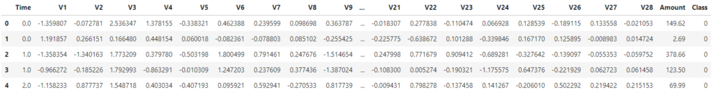
We will use a Kaggle dataset about credit card fraud detection. This dataset consists of transactions made by credit cards in September 2013 by European cardholders. It contains 492 frauds out of a total of 284,807 transactions. You can see that it is highly unbalanced, where the positive class (frauds) account for 0.172% of all transactions.
The objective of this article is to illustrate how to train a built-in model like XGBoost in an AWS Sagemaker’s notebook instance. In this case supervised learning, specifically a binary classification problem.
But first, what do I mean by built-in algorithms? Amazon SageMaker provides several built-in algorithms that you can use to train your models. These algorithms are highly optimized, scalable, and designed to generate accurate models rapidly, eliminating the need to create and maintain the underlying algorithm containers, thus saving time and resources.
Let’s start by importing the basic python libraries. We will use pandas to read the dataset:
Python
import pandas as pd
import numpy as np

# Load dataset
df = pd.read_csv('creditcard.csv')
We should do an Exploratory Data Analysis here, however, we will skip it for brevity. We will drop the feature “Time” and will retain the rest of the anonymised credit-card-related features. Also, let’s check the number of transactions belonging to each class (Fraud or Normal):
Python
# Drop Time column
df = df.drop(columns=['Time'])

# Check number of transactions of each type
df.Class.value_counts()
0    284315
1       492
Name: Class, dtype: int64
It is heavily imbalanced. Since this article aims to focus on the Sagemaker side, we won’t try to optimise the model to get the best possible result. Therefore, let’s just undersample randomly the majority class. We will take randomly the same number of transactions that we have in the normal ones, i.e. 492.
Python
# Fraud transactions
df_1 = df[df.Class == 1]

# Undersampled normal transactions
df_0 = df[df.Class == 0].sample(df_1.shape[0])
Now we concatenate both datasets and reset the index:
Python
df_bal = pd.concat((df_0, df_1), axis=0)
df_bal.reset_index(drop=True, inplace=True)
Before continuing, since we are going to use XGBoost, which is a decision-tree-based algorithm, we don’t necessarily need to scale the features.
First, we need to split into features (X) and target (y).
Python
X = df_bal.iloc[:,:-1]
y = df_bal.iloc[:,-1]
Now, using sklearn function train_test_split, we can split our data into the training and testing sets.
Python
from sklearn.model_selection import train_test_split

X_train, X_test, y_train, y_test = train_test_split(X,
                                                    y,
                                                    test_size=0.10,
                                                    random_state=42,
                                                    stratify=y,
                                                    )
We use 10% of the data as a testing set. Also, note that we use the argument stratify. This is to ensure that each set contains approximately the same percentage of samples of each target class as the complete set (y).
Since we want a validation set too, we will further split the training set. Again allocating 10%, this time as validation.
Python
X_train, X_val, y_train, y_val = train_test_split(X_train,
                                                  y_train,
                                                  test_size=0.1,
                                                  random_state=42,
                                                  stratify=y_train
                                                  )
We can have a look at the size of each set to verify that we have carried that over correctly.
Python
X_train.shape[0], X_test.shape[0], X_val.shape[0]
(885, 99, 89)
Amazon S3 bucket, part of AWS’s Simple Storage Service (S3), is a scalable cloud storage solution providing object storage, allowing users to store and retrieve data in units termed as objects, instead of traditional file systems. Each object within the S3 bucket is identified with a unique, user-assigned key, ensuring precise data retrieval.
We will create an S3 bucket where we will store our model files. The prefix refers to the subdirectories or subfolders where the files will be.
Python
bucket = 'sagemaker-bucket'
prefix = 'data'
Sagemaker built-in algorithms require datasets where the first feature is the label or target (y) and the rest are independent variables (X). For the training and validation sets to be used by the algorithms, we need to upload them to an S3 bucket in a special way.
First, let’s create a Sagemaker session in this notebook:
Python
import sagemaker
sess = sagemaker.Session()
We need to concatenate the y and X to create the dataset in the expected format and order and save it locally as a CSV file. Afterwards, we need to upload it to a specific S3 bucket:
Python
# Training set
pd.concat([y_train, X_train], axis=1).to_csv('train.csv',
                                             index=False,
                                             header=False)
sess.upload_data(path='train.csv',
                 bucket=bucket,
                 key_prefix=prefix+'/train')

# Validation set
pd.concat([y_val, X_val], axis=1).to_csv('validation.csv',
                                         index=False,
                                         header=False)
sess.upload_data(path='validation.csv',
                 bucket=bucket,
                 key_prefix=prefix+'/validation')
Next, we use the Sagemaker’s TrainingInput class to configure a data input flow for training and validation:
Python
from sagemaker.inputs import TrainingInput

# Training set
s3_input_train = TrainingInput(s3_data=f's3://{bucket}/{prefix}/train',
                               content_type='csv')

# Validation set
s3_input_validation = TrainingInput(s3_data=f's3://{bucket}/{prefix}/validation/',
                                    content_type='csv')
Time to train our model. In this stage, we need to import our built-in algorithm.
Before that, we will need the following information:
- region: the AWS Region where the SageMaker notebook instance runs (eu-west-2, eu-central-1, us-east-1…).
- session: the SageMaker session that holds the configuration and is used to create all the needed AWS resources like training jobs, endpoints, etc.
- role: the IAM Role ARN is used to give training and deployment access to your data. You usually get this role when you create a notebook instance unless specified otherwise.
- instance type: is the type of EC2 instance used for training your model, such as “ml.m4.xlarge”, “ml.m5.large”, etc. You’ll need to carefully choose the optimal for your case, checking parameters like memory, CPU and, of course, price per hour.
Python
import boto3

region = boto3.Session().region_name
role = sagemaker.get_execution_role()
instance_type = 'ml.m4.large'
Next, we need to retrieve the container image URI for the specified built-in algorithm or model, in this case, XGBoost. Each built-in algorithm or pre-built model in SageMaker is stored in a Docker container, and this container is located at a specific URI (Uniform Resource Identifier).
When you are creating an estimator, you need to specify the location (URI) of the Docker container that has the algorithm or model. The image_uris.retrieve function simplifies this process by generating the correct URI for you based on the algorithm or model, region, and other parameters you specify.
Python
container = sagemaker.image_uris.retrieve(framework="xgboost",
                                          region=region,
                                          version="latest"
                                          )
An Estimator is an abstraction represented by the Estimator class in the SageMaker Python SDK, which allows users to train machine learning models. It encapsulates the training job and its associated configurations, such as the algorithm container, training data, hyperparameters, and compute resources.
Python
from sagemaker.estimator import Estimator

xgb = Estimator(container,
                role,
                sagemaker_session=sess,
                instance_count=1,
                instance_type=instance_type,
                input_mode='File',
                output_path=f's3://{bucket}/{prefix}/output',
                train_use_spot_instance=True
                )
Let’s explain some of the arguments we set:
- instance_count: The number of Amazon EC2 instances you want to use for training. 1 indicates a single instance.
- input_mode: The input mode that the algorithm supports. “File” mode means the training data is transferred to the training instances using Amazon S3.
- output_path: The S3 location for saving the training results (model artifacts and output files).
- train_use_spot_instance: This argument suggests using EC2 Spot Instances for training, which can significantly reduce the cost of training models.
We need to set up also the hyperparameters. These are some of the hyperparameters you can set up:
- alpha: The L1 regularization term on weights, used to avoid overfitting.
- eta: The learning rate, controlling the contribution of each tree in the ensemble.
- gamma: The minimum loss reduction required to make a further partition on a leaf node of the tree.
- max_depth: The maximum depth of a tree, controlling overfitting.
- min_child_weight: The minimum sum of instance weight needed in a child, used to control overfitting.
- subsample: The fraction of training data to randomly sample in each round to prevent overfitting.
- objective: The learning task and the corresponding learning objective. Here, we chose binary classification with logistic regression.
- num_round: The number of boosting rounds or trees to build, equivalent to the number of models in the ensemble.
Python
xgb.set_hyperparameters(alpha=1.5,
                        eta=0.1,
                        gamma=4,
                        max_depth=2,
                        min_child_weight=3,
                        subsample=0.8,
                        objective='binary:logistic',
                        num_round=100,
                        )
Finally, time to fit our data:
Python
xgb.fit({'train': s3_input_train,
         'validation': s3_input_validation})
2023-09-23 15:28:25 Starting - Starting the training job...
2023-09-23 15:28:51 Starting - Preparing the instances for trainingProfilerReport-1695396505: InProgress
[...]
[15:31:01] src/tree/updater_prune.cc:74: tree pruning end, 1 roots, 6 extra nodes, 0 pruned nodes, max_depth=2
[0]#011train-error:0.080226#011validation-error:0.033708
[15:31:01] src/tree/updater_prune.cc:74: tree pruning end, 1 roots, 6 extra nodes, 0 pruned nodes, max_depth=2
[1]#011train-error:0.080226#011validation-error:0.067416
[15:31:01] src/tree/updater_prune.cc:74: tree pruning end, 1 roots, 6 extra nodes, 0 pruned nodes, max_depth=2
[2]#011train-error:0.079096#011validation-error:0.089888
[15:31:01] src/tree/updater_prune.cc:74: tree pruning end, 1 roots, 6 extra nodes, 0 pruned nodes, max_depth=2
[...]
...
2023-09-23 15:31:17 Uploading - Uploading generated training model
2023-09-23 15:31:17 Completed - Training job completed
Training seconds: 102
Billable seconds: 102
Time to deploy the trained model so it can be used in production. We need to select the instance type and count depending on our requirements. Also the model and endpoint names:
Python
# Set model and endpoint names
model_name = 'sagemaker-fraud-detection'

# create endpoint and predictor
xgb_predictor = xgb.deploy(initial_instance_count=1,
                           instance_type=instance_type,
                           model_name=model_name,
                           endpoint_name=model_name,
                           )
-----!
Before getting the predictions, we need to specify the serialization format that the SageMaker Predictor will use when sending data to our model endpoint. In this case, we’ll be using the CSVSerializer, meaning that the predictor will serialize the input data to CSV format before sending it to the model endpoint for inference. Serialization is the process of converting a data structure or object state into a format that can be easily stored or transmitted, and subsequently reconstructed. In other words, it’s about translating complex data types such as objects or structures into a format (like a string) that can be easily rendered into a file, sent over the network, or saved into a database. Once the serialized data reaches its destination, it can be deserialized back into its original format.
Python
from sagemaker.predictor import CSVSerializer
xgb_predictor.serializer = CSVSerializer()
Time to get the predictions for our testing set. We use the method predict of our deployed predictor. However, this method requires the data to be in a numpy array format, not in a pandas Dataframe. Finally, we need to decode the output and convert it to numpy array.
Python
predictions = xgb_predictor.predict(X_test.values)
y_pred = np.fromstring(predictions.decode('utf-8'), sep=',')
Now we can assess the performance of the model. Since our test data was balanced at the beginning, we will calculate the accuracy for simplicity.
Python
accuracy = (y_pred.round() == y_test).sum() / y_test.shape[0] * 100
print(f'The accuracy of the model is {accuracy:.2f}%')
The accuracy of the model is 94.95%
We can also see the confusion matrix:
Python
from sklearn.metrics import confusion_matrix

conf_matrix = confusion_matrix(y_test, y_pred.round())
print(conf_matrix)
[[49  1]
 [ 4 45]]
This was a toy dataset and it was possibly highly preprocessed. Therefore it was to expect a very good result.
Imagine you created your model and endpoint in the past and you want to test some data in a notebook. You could load your endpoint in a predictor and do the same as we’ve just done when assessing the performance.
Python
from sagemaker.predictor import Predictor

# Load endpoint
predictor = Predictor(endpoint_name=model_name)

# Set serialization to CSV
predictor.serializer = CSVSerializer()
Get the predictions as done before:
Python
predictions = predictor.predict(X_test.values)
y_pred = np.fromstring(predictions.decode('utf-8'), sep=',')
The next step would be to make the endpoint available for a production environment. You can achieve this using an AWS Lambda Function and creating an API from it. We will cover this in future articles.
Post Views: 132