Example on how to extract and plot fitness diversity for a population, hall of fame, or frontier using histogram and probability curves. From question https://groups.google.com/forum/#!topic/deap-users/Y8JX4AKwzhk

deap_diversity_plot.py

# Examples on how to extract and plot fitness diversity for a population, hall of fame, or 
#     frontier using histogram and probability curves. Mostly working with multi objective fitness as per
#     question from https://groups.google.com/forum/#!topic/deap-users/Y8JX4AKwzhk
# Derek M Tishler - 2019

import array
import random


import numpy as np
import matplotlib as mpl
mpl.use('Agg') # may need to remove this if using plt.show()
import matplotlib.pyplot as plt

from scipy import stats

from deap import algorithms
from deap import base
from deap import creator
from deap import tools



def plot_diversity(hof):

    fig = plt.figure(figsize=(8,4), dpi=200)

    n_row = 1
    n_col = len(hof[0].fitness.values)

    # Loop over the diff fitness dimensions and plot a histogram and probability curves
    for fit_tuple_idx in range(n_col):

        ax = plt.subplot2grid((n_row,n_col), (0, fit_tuple_idx), rowspan=1)

        # hof or paretofrontier is list of top or non-dominating front, either way its a list of individuals you can get fitness from
        #example: hof[0].fitness.values
        # so we can iteratare over the list and get the fitness, then plot histograms or any method you like to explore convergence 
        fitnesses = [ind.fitness.values[fit_tuple_idx] for ind in hof]

        # lets plot a histogram of each fitness(or just the 1 if its not multi objective)
        n,bins,patches = ax.hist(fitnesses, histtype='stepfilled', bins=40, color='forestgreen' ,alpha=0.2, weights=np.ones_like(fitnesses)/float(len(fitnesses)))

        # To form a proba curve on the data i use numpy histogram for convenience and to ensure scaling for bin are readable for probabilities 
        n, bin_edges = np.histogram(fitnesses, bins=40, density=True)
        norm_factor  = 1./float(n.sum())

        # now, also form a gauss kde on the DATA then scale to match the hist
        # note can increase the multipliers here and get a kde that falls to zero on endges, but its personal preff
        x_grid               = np.linspace(np.min(fitnesses)-0.*np.std(fitnesses), np.max(fitnesses)+0.*np.std(fitnesses), 1000) 
        kde_sample_evaluated = stats.gaussian_kde(fitnesses, bw_method=0.125).evaluate(x_grid)
        ax.plot(x_grid, kde_sample_evaluated*norm_factor, c='forestgreen', alpha=0.3, lw=0.6)

        ax.set_ylabel('probability')
        ax.set_xlabel(r'fitness$_{ %d}$'%(fit_tuple_idx+1))
        ax.grid()

    plt.tight_layout()
    #plt.show(True)
    plt.savefig('hof_diversity.png')
    plt.close()




def plot_scatter_w_diversity(hof, ext_ind_f=None, ext_ind_l=None):

    if ext_ind_f is not None:
        hof = [ext_ind_f] + hof
    if ext_ind_l is not None:
        hof = hof + [ext_ind_l]

    fig = plt.figure(figsize=(8,4), dpi=200)

    ax = plt.subplot2grid((1,2), (0, 0), rowspan=1)

    x = [float(ind.fitness.values[0]) for ind in hof]
    y = [float(ind.fitness.values[1]) for ind in hof]

    # labels to marry with figure in source whitepaper
    plt.text(x[0]-5., y[0]+1., "ext", fontsize=5,
            horizontalalignment='center', verticalalignment='center')
    plt.text(x[-1]-5., y[-1]-0.5, "ext", fontsize=5,
            horizontalalignment='center', verticalalignment='center')

    plt.text(x[0]+(x[0+1]-x[0])/2. - 3., y[0]+(y[0+1]-y[0])/2. + 2., r'd$_f$', fontsize=5,
            horizontalalignment='center', verticalalignment='center')
    plt.text(x[-1]+(x[-1]-x[-2])/2. - 3., y[-1]+(y[-2]-y[-1])/2. + 0., r'd$_l$', fontsize=5,
            horizontalalignment='center', verticalalignment='center')
    for i in range(1,len(x[1:-1])):
        plt.text(x[i]+(x[i+1]-x[i])/2. - 3., y[i]+(y[i+1]-y[i])/2. + 1., r'd$_{%d}$'%i, fontsize=5,
            horizontalalignment='center', verticalalignment='center')

    plt.scatter([x[0]],[y[0]], s=8, c='w', alpha=0.75, edgecolors='forestgreen', linewidth=1.0)
    plt.scatter([x[-1]],[y[-1]], s=8, c='w', alpha=0.75, edgecolors='forestgreen', linewidth=1.0)
    plt.scatter(x[1:-1],y[1:-1], s=8, c='forestgreen', alpha=0.75)
    plt.plot(x,y, lw=0.75, c='forestgreen', alpha=0.75)
    plt.grid()




    

    # https://www.iitk.ac.in/kangal/Deb_NSGA-II.pdf
    equation_1_page_188_str = r'$\Delta = \dfrac{d_f + d_l + \sum_{i=1}^{N-1} \left| d_i - \bar{d} \right|}{d_f + d_l + (N-1){\bar{d}}}$'
    def equation_1_page_188(hof):
        # assuming end points are extreme solutions(use a big pop for good data)
        d_l   = np.linalg.norm(np.array(hof[-1].fitness.values)-np.array(hof[-2].fitness.values))
        d_f   = np.linalg.norm(np.array(hof[1].fitness.values)-np.array(hof[0].fitness.values))
        N     = float(len(hof))
        d_i   = np.abs([np.linalg.norm(np.array(ind.fitness.values)-np.array(hof[i+2].fitness.values)) for i,ind in enumerate(hof[1:-2])])
        d_bar = np.mean(d_i)
        sum_  = np.sum([d-d_bar for d in d_i])

        diversity_measure_del = (d_f + d_l + sum_)/(d_f + d_l + (N-1.)*d_bar)

        return diversity_measure_del

    diversity_measure_del = equation_1_page_188(hof)

    ax = plt.subplot2grid((1,2), (0, 1), rowspan=1)
    plt.text(0.5,0.7, equation_1_page_188_str, fontsize=17,
        horizontalalignment='center', verticalalignment='center', transform=ax.transAxes)
    plt.text(0.5,0.25, r"$\Delta = $%0.3f"%diversity_measure_del, fontsize=20,
        horizontalalignment='center', verticalalignment='center', transform=ax.transAxes)
    plt.axis('off')

    plt.tight_layout()
    #plt.show(True)
    if ext_ind_f is not None or ext_ind_l is not None:
        plt.savefig('hof_frontier_estimated_extreme.png')
    else:
        plt.savefig('hof_frontier.png')
    plt.close()




########## Can ignore this section, and replace with hof or pop list ##########
# I create a fake pop with fitness values matchin the question's
creator.create("FitnessMax", base.Fitness, weights=(1.0,1.0))
creator.create("Individual", array.array, typecode='b', fitness=creator.FitnessMax)

toolbox = base.Toolbox()

# Attribute generator
toolbox.register("attr_bool", random.randint, 0, 1)

# Structure initializers
toolbox.register("individual", tools.initRepeat, creator.Individual, toolbox.attr_bool, 100)
toolbox.register("population", tools.initRepeat, list, toolbox.individual)




hof_fit_to_force = [
    (173.384071,100.0),
    (45.082696,80.0),
    (34.562327,79.0),
    (24.557862,68.0),
    (14.550288,50.0),
    (13.726517,33.0),
    (13.479549,24.0),
    (13.439238,23.0),
    (13.430936,22.0),
    (13.409498,20.0),
    (9.029356,19.0),
    (7.88063,18.0),
    (2.611496,7.00),
]

hof = toolbox.population(n=len(hof_fit_to_force))

for h,f in zip(hof, hof_fit_to_force):
    h.fitness.values = f
# oversample original data
#hof = toolbox.population(n=10000)
#for h in hof:
#    h.fitness.values = [(x+((np.random.random()-0.5)*x),y+((np.random.random()-0.5)*y)) for x,y in [random.choice(hof_fit_to_force),]][0]

# Done setting up for example, in your code you just use below and reference hof or pop
###########################################################################


plot_diversity(hof)

plot_scatter_w_diversity(hof)

# if we have a method to est the extreme points, we can create 2 new inds and fill their fit with these estimates
# lets split the hof in half, and build a std on each side to mimic asymetric distribution
ext_sol_f = (hof[0].fitness.values[0]+np.std([ind.fitness.values[0] for ind in hof[:len(hof)/2]]), hof[0].fitness.values[1]+np.std([ind.fitness.values[1] for ind in hof[:len(hof)/2]]))
ext_sol_l = (hof[-1].fitness.values[0]-np.std([ind.fitness.values[0] for ind in hof[-len(hof)/2:]]), hof[-1].fitness.values[1]-np.std([ind.fitness.values[1] for ind in hof[-len(hof)/2:]]))

ext_ind_f = toolbox.individual()
ext_ind_f.fitness.values = ext_sol_f

ext_ind_l = toolbox.individual()
ext_ind_l.fitness.values = ext_sol_l

# override values will append to start and finish of hof. not very general but we know frontier shape?
plot_scatter_w_diversity(hof, ext_ind_f=ext_ind_f, ext_ind_l=ext_ind_l)

Resulting in a saved figure:

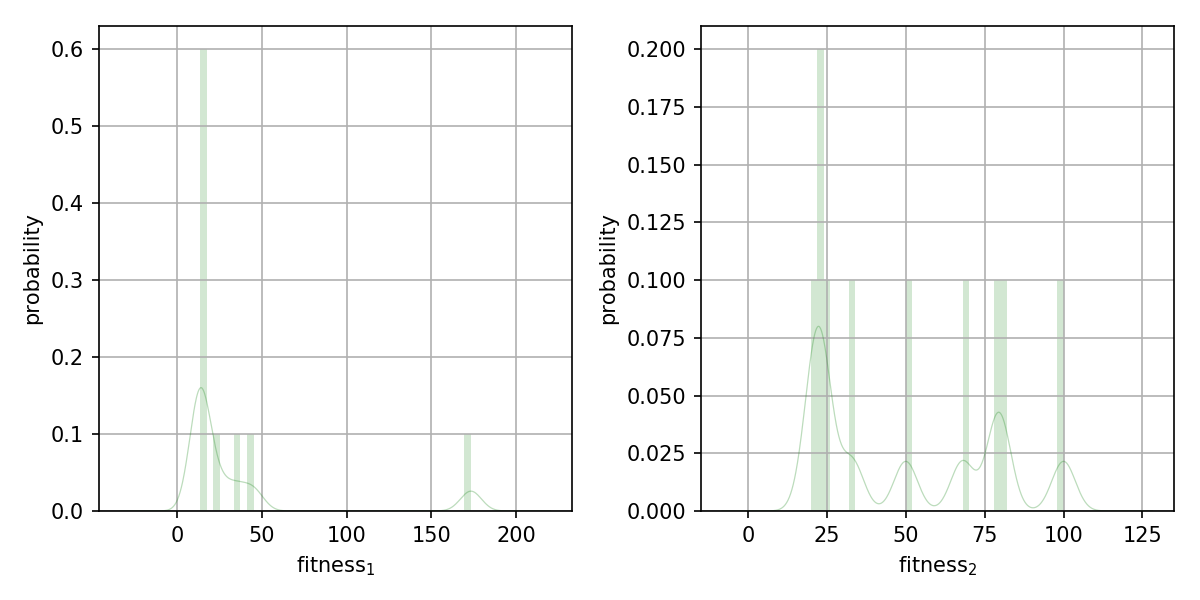
First chart is with a wider limit on the kde plot...with the default multiplier of 0. you would normally see the following figure:
So above is:
x_grid = np.linspace(np.min(fitnesses)-1.*np.std(fitnesses), np.max(fitnesses)+1.*np.std(fitnesses), 1000)
vs below's:
x_grid = np.linspace(np.min(fitnesses)-0.*np.std(fitnesses), np.max(fitnesses)+0.*np.std(fitnesses), 1000)

With some random over sampling of your data to mimic a much larger pop, we can see what the chart can potentially show:

Now can attempt to measure diversity, without a benchmark, via diversity metric del found in paper:
A Fast and Elitist Multiobjective Genetic Algorithm: NSGA-II
Kalyanmoy Deb, Associate Member, IEEE, Amrit Pratap, Sameer Agarwal, and T. Meyarivan
https://www.iitk.ac.in/kangal/Deb_NSGA-II.pdf

Example of the frontier diversity plot generated by script:

Updated code with correction to diversity calc after noticing issues once labels were added to match whitepaper:

Code updated with an example of adding an estimated extreme point(s) vs using the first/last item in hof like before. Messy but can help with quick solution to current need to compare 2 hofs on file for questioner.