Last active
September 6, 2019 13:25
-
-
Save FilipDominec/9ab21b7eecb1875fcb2eba9958791cc1 to your computer and use it in GitHub Desktop.
Playground for visualisation of the Schrödinger equation solutions in one dimension
This file contains bidirectional Unicode text that may be interpreted or compiled differently than what appears below. To review, open the file in an editor that reveals hidden Unicode characters.
Learn more about bidirectional Unicode characters
| #!/usr/bin/python3 | |
| import matplotlib.pyplot as plt | |
| import numpy as np | |
| import numpy.linalg as la | |
| width, n= 1., 500 ## width of the 1D quantum system, and number of points | |
| nplot = 10 ## number of quantum states to plot | |
| h = 1e-4 ## our definition of "Planck constant" determines the density of states | |
| psiscale = .01 ## for plotting only: approximate matching of probability and potential scales | |
| x = np.linspace(-width/2,width/2,n) ## horizontal axis | |
| def laplace(n): return (-np.roll(np.eye(n),1) + 2*np.eye(n) - np.roll(np.eye(n),-1))*n**2 ## create off-diagonal elements | |
| V = ((x+.01)**4)*100 - (x-.01)**2 * 10 + .2 ## arbitrary potential (with two asymmetric minima) | |
| H = laplace(n) * h + np.diag(V) ## Hamiltonian consists of kinetic and potential terms | |
| Es, psis = la.eigh(H) ## the actual eigenfunction computation | |
| fig, ax = plt.subplots(1,1) | |
| for psi, E in zip(psis.T[:nplot], Es[:nplot]): | |
| psi /= (np.sum(psi**2)/n * width)**.5 ## normalize wavefunction to one | |
| ax.fill_between(x, E+psi**2*psiscale, E*np.ones_like(psi), color='silver') | |
| plt.plot(x, E+psi**2*psiscale, label='$\\psi^2$', ) | |
| plt.plot(x, E*np.ones_like(psi), label='$E$', c='k') | |
| ## If psi is eigenvector, this should be identical: | |
| #plt.plot(x, E+E *psi , label='$E \\psi$', c='r', lw=2) | |
| #plt.plot(x, E+np.dot(H,psi), label='$\\hat H\\psi$', c='g') | |
| plt.plot(x[V<E], (V)[V<E], label='$V$', c='k', ls=':') ## potential | |
| plt.xlabel(u"Position"); plt.ylabel(u"Energy levels; Wavefunction probability"); plt.grid() | |
| plt.savefig("output.png", bbox_inches='tight') | |
| #plt.show() |
Sign up for free
to join this conversation on GitHub.
Already have an account?
Sign in to comment
Typical output for an asymmetrical quantum well follows:
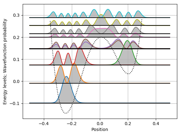
First, the left valley is filled with the first and second wavefunction which resemble the first two states of a harmonic oscillator. The following three pairs of states show that the phenomenon of ''state hybridization'' requires the coupling to be not too weak and also not too strong:
For this choice of the potential, the third (green line) and fourth (red line) states by coincidence (...or my choice of potential function) have a very close energetic level; however, at this level, the coupling between the left and right wells is so weak that we observe no hybridisation. One state is concentrated in the left valley, the other in the right valley.
The situation changes at higher energy, which enables increased quantum tunneling between the wells. Thus, the fifth and sixth states are hybridized - they have quite similar profile of probability density as obvious from the plots, yet they differ by the mutual phase of their left and right parts (known as "bonding" vs. "antibonding" states, which is not shown in the plots).
The seventh (pink) and eighth (grey) states are coupled yet stronger than the previous two. It has a similar impact on their wavefunction shapes, but now even the probabilities obviously differ, and it leads also to appreciable energy splitting.
The sequence of all higher states is similar to the linear harmonic oscillator, except for the potential growing with the 4th power of ''x''.