Loads ASCII-exported spectra from Princeton spectrometer, exports "worm plot" of spectral position and intensity of the peak

multifit.py

#!/usr/bin/python3
#-*- coding: utf-8 -*-

"""
Batch fitting of multiple spectra - evaluation of spectroscopic response of InGaN/GaN quantum-well sensors to the 
presence of surface charges induced by gases or liquids.

Invocation:
    ./multifit.py   <filename>.dat
where
    filename    =   ASCII data file to be processed, in the format exported by Princeton monochromator of four columns
                    corresponding to: 0. wavelength, 1. numbering of spectral acquisition, 2. nothing, 3. rel. intensity

Output:
    <filename>contours.png  
                =   spectrum as background contours, detected emission energy as black line
    <filename>_fit.txt
                =   fitting results: n,    Ifit, E0fit, FWHMfit, Ip, Ep,  Is,Ecom,  
                    n - number of spectrum
                    Ifit, E0fit, FWHMfit - fitting results, see fitting function in the code below
                    Ip, Ep - intensity and energy of 'peak point', i.e. absolute maximum
    <filename>_worms.png
    <filename>_worms.pdf
                =   the worm plot                   Is, Ecom - summed intensity and center-of-mass position

"""

## Import common moduli
import matplotlib, sys, os, time
from pathlib import Path
import matplotlib.pyplot as plt
import numpy as np
from scipy.constants import c, hbar, pi

## ========== User settings ===========

## Single-Gaussian fitting, similar as above, but no phonon replicas (samples differ by their spectra from the model)
##   I      - peak integral intensity
##   E0     - central energy
##   FWHM   - full width at half maximum of the major peak
##   R      - describe the ratio of consecutive LO-phonon replicas in GaN, each red-shifted by 0.092 eV
def fit_func(E, I, E0, FWHM):
    return  I/FWHM*     np.exp(-(E-E0)**2/(FWHM/2)**2 * np.log(2))
fit_bounds   = ([0, 1240/490, .001],   [1e7, 1240/420, .4])
file_note = ''

## Plotting options
worm_yscale = 'log'    # Logarithmic intensity axis for wormplots may better enable to compare sample evolution
ylim = (2.4, 2.95)      # Energy limits for plotting (just visual)

## Spectral clipping to the visible region (clips actual data - affects fitting)
clipcenter, clipwidth = (ylim[0]+ylim[1])/2, (ylim[1]-ylim[0])   # note: use high value for clipwidth to disable clipping

## Debugging options: 
limit_number_of_spectra = False            # set to False to process spectra up to the end
pick_each_nth_spectrum = 1              # use 1 to process each spectrum
debugmode = False                       # Will also export a diagnostics of the selected spectral fit


## Experimental features for future
flatten_rel_file_path = False
subtract_background = False   # experimental!

## Experimental: uncomment for double-peak fitting (may need fine-tuning to converge!)
#def fit_func(E, I, E0, FWHM, I2, DeltaE, FWHM2): ## Experimental
    #return   I /FWHM*  np.exp(-(E       -E0)**2/(FWHM /2)**2 * np.log(2))    + \
             #I /FWHM * np.exp(-(E       -E0)**2/(FWHM /2)**2 * np.log(2))
#fit_bounds   = ([0, 2.7, .001, 0, 0.05, .001],   [1e6, 2.9, .3, 1e6, 0.25, .2])
#file_note = 'double_gaussian'

## ========== End of user settings ===========




## Three different plotting functions
def plot_diagnostic():
    fig = plt.figure(); ax = plt.subplot(111)
    plt.plot(energy_eV, intensity, 'b-') # The measured spectrum
    if 'file_note' != 'double_gaussian':
        plt.plot(energy_eV, fit_func(energy_eV, *popt), 'g--', label='fit: I=%5.3f, E0=%5.3f, FWHM=%5.3f' % tuple(popt))
    else :
        ax.plot(energy_eV, fit_func(energy_eV, *popt), 'k--', 
                label='fit: I=%5.3f, E0=%5.3f, FWHM=%5.3f, I=%5.3f, E0=%5.3f, FWHM=%5.3f' % tuple(popt))
        popt2 = popt.copy();  popt2[0]= 0       # First Gaussian separately
        ax.plot(energy_eV, fit_func(energy_eV, *popt2), 'r--', 
                label='fit: I=%5.3f, E0=%5.3f, FWHM=%5.3f, I=%5.3f, E0=%5.3f, FWHM=%5.3f' % tuple(popt))
        popt2 = popt.copy(); popt2[3]= 0        # Second Gaussian separately
        ax.plot(energy_eV, fit_func(energy_eV, *popt2), 'g--', 
                label='fit: I=%5.3f, E0=%5.3f, FWHM=%5.3f, I=%5.3f, E0=%5.3f, FWHM=%5.3f' % tuple(popt))
        #fig.title(popt) # todo
    plt.savefig(outfilename + file_note + '_fit_diagnostic{:}.png'.format(num))
    #plt.show()


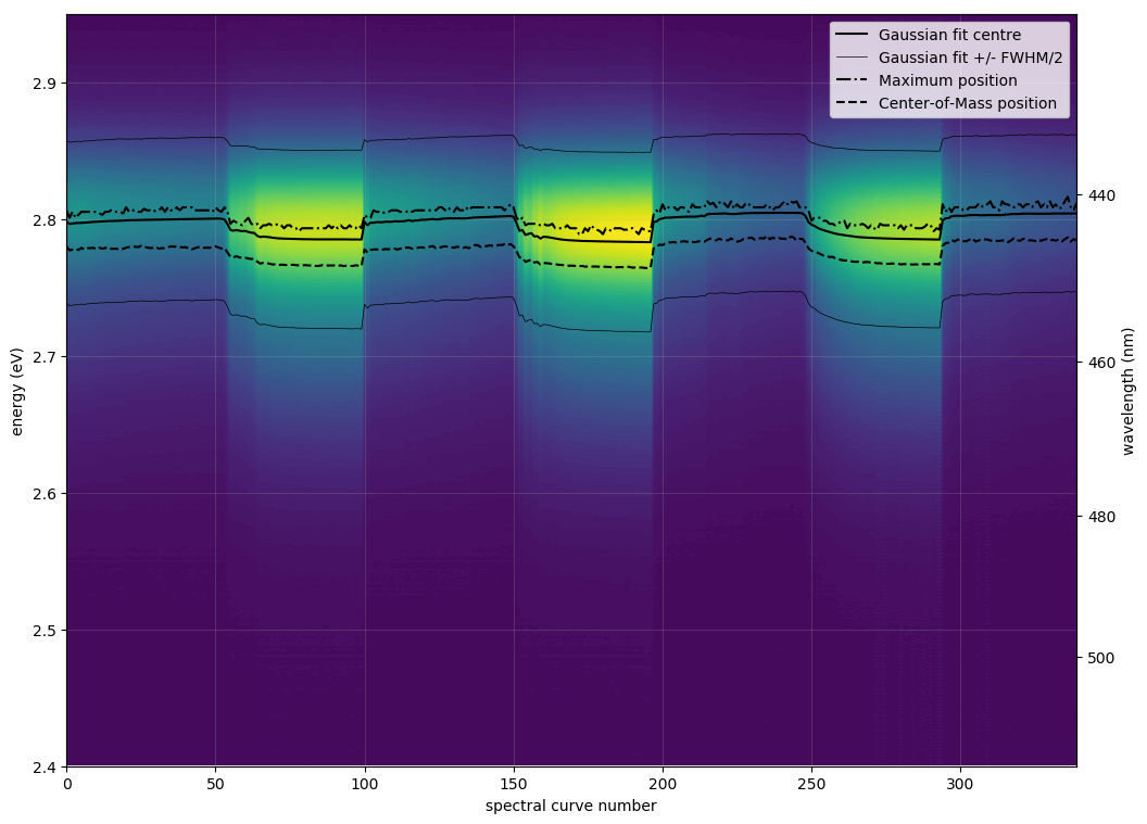
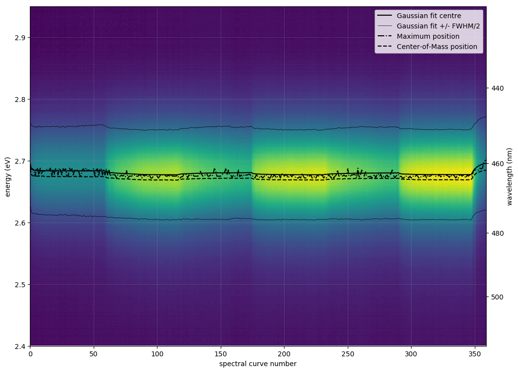
def plot_all_spectra_2D():
    fig, ax = plt.subplots(figsize=(12, 9))
    ax.contourf(np.arange(n_spec)[:num+1], energy_eV, intensities[:num+1,:].T, levels=np.linspace(np.min(intensities), np.max(intensities), 100))
    ax.plot(np.arange(n_spec)[:num+1:], results_for_file[:,2], ls='-', c='k', label='Gaussian fit centre')
    ax.plot(np.arange(n_spec)[:num+1], results_for_file[:,2]+results_for_file[:,3]/2, ls='-', c='k', lw=.5, label='Gaussian fit +/- FWHM/2')
    ax.plot(np.arange(n_spec)[:num+1], results_for_file[:,2]-results_for_file[:,3]/2, ls='-', c='k', lw=.5, label='')
    ax.plot(np.arange(n_spec)[:num+1], results_for_file[:,5], ls='-.', c='k', label='Maximum position')
    ax.plot(np.arange(n_spec)[:num+1], results_for_file[:,7], ls='--', c='k', label='Center-of-Mass position')
    if ylim: plt.ylim(ylim) # Force y-limit of plotting 
    plt.grid(alpha=.2)  
    plt.xlabel(u"spectral curve number"); 
    plt.ylabel(u"energy (eV)"); 
    plt.legend(prop={'size':10}, loc='upper right')

    ## This is an optional ugly hack to get a secondary y-axis for wavelength
    def right_tick_function(p): return 1240/p
    ax2 = ax.twinx()
    ax2.set_ylim(np.array(ax.get_ylim()))
    ax2.set_ylabel('wavelength (nm)')
    ## If we wish nice round numbers on the secondary axis ticks...
    right_ax_limits = sorted([right_tick_function(lim) for lim in ax.get_ylim()])
    yticks2 = matplotlib.ticker.MaxNLocator(nbins=20, steps=[1,2,5]).tick_values(*right_ax_limits)
    ## ... we must give them correct positions. To do so, we need to numerically invert the tick values:
    from scipy.optimize import brentq
    def right_tick_function_inv(r, target_value=0): 
        return brentq(lambda r,q: right_tick_function(r) - target_value, ax.get_ylim()[0], ax.get_ylim()[1], 1e6)
    valid_ytick2loc, valid_ytick2val = [], []
    for ytick2 in yticks2:
        try:
            valid_ytick2loc.append(right_tick_function_inv(0, ytick2))
            valid_ytick2val.append(ytick2)
        except ValueError:      ## (skip tick if the ticker.MaxNLocator gave invalid target_value to brentq optimization)
            pass
    ax2.set_yticks(valid_ytick2loc)  ## Finally, we set the positions and tick values
    from matplotlib.ticker import FixedFormatter
    ax2.yaxis.set_major_formatter(FixedFormatter(["%g" % righttick for righttick in valid_ytick2val]))

    figure_name = outfilename+file_note+'_contours.png'
    gprint("    2D spectral data plotted to " + figure_name + '\n')
    fig.savefig(outfilename+file_note+'_contours.png', bbox_inches='tight')
    fig.savefig(outfilename+file_note+'_contours.pdf', bbox_inches='tight')

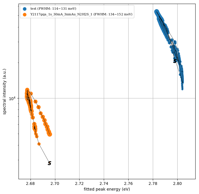
def plot_worm(results_for_batch, labels):
    clip = 0
    step = 1
    fig = plt.figure(figsize=(8,8)); ax = plt.subplot(111)
    matplotlib.rc('font', size=12, family='serif')

    for results_for_file, label in zip(results_for_batch, labels):
        ny = results_for_file[clip::step,1]  # intensity
        nx = results_for_file[clip::step,2]  # spectral position
        w  = results_for_file[clip::step,3]  # spectral width
        nw = w-np.min(w)*0.99 # remember spectral width intensity

        ll = "%s" % (label.replace('0s','0185ms').replace('FWHM','').split('.dat')[0]) + \
                 (" (FWHM: {:3.0f}$-${:3.0f} meV)".format(np.min(w[clip:])*1e3,np.max(w[clip:])*1e3))
        if 'NOLABEL' in ll: 
          ll = ''
        else:
          ll = ll.rsplit('/',1)[-1].replace(' fit.txt','').replace('.txt','')
        ax.scatter(nx, ny, label=ll, s=120*nw/np.max(nw), marker='o', alpha=1)
        ax.scatter(nx[0], ny[0], label="", color='k', s=80, marker='$s$', alpha=1)
        ax.plot(nx, ny, label="", lw=.5, c='k')

    if worm_yscale == 'log':
        ax.set_yscale('log')
    else:
        globmin = min(np.min(yy) for yy in ys[::3]) 
        globmax = max(np.max(yy) for yy in ys[::3])
        if globmin < 0.5*globmax: ax.set_ylim(ymin=0)

    ax.set_xlabel("fitted peak energy (eV)")
    ax.set_ylabel("spectral intensity (a.u.)")
    #plot_title = sharedlabels[-6:] ## last few labels that are shared among all curves make a perfect title
    ax.set_title('', fontsize=10) 
    ax.legend(loc='best', prop={'size':8})
    ax.grid(True)

    plt.savefig(outfilename + file_note + '_worms.png', bbox_inches='tight') # todo switch from plt. to fig.
    plt.savefig(outfilename + file_note + '_worms.pdf', bbox_inches='tight')


## User interaction  
if len(sys.argv) == 1:      # if no parameters given, enter the interactive GUI mode
    from tkinter import filedialog
    from tkinter import *
    root = Tk()
    root.title('multifit.py processing report') 
    T = Text(root, height=20, width=150)
    T.pack()
    filenames = filedialog.askopenfilenames(initialdir = os.getcwd(),
            title = "Select spectral data file to be processed, please",
            filetypes = (("DAT files","*.dat"),("all files","*.*")))
else: 
    T = None
    filenames = sys.argv[1:]

def gprint(*args, **kwargs):    # printing in the stdout and possibly into the window
    if T: 
        T.insert(END, ' '.join(args)+'\n') 
        root.update()
    print(*args, **kwargs)

## Load and delinearize the spectral data (according to spectrum numbering in the 3rd column of the DAT file)
results_for_batch, names_for_batch = [], []
for filename in filenames:
    gprint("Processing", filename)
    outfilename = filename.replace('.dat', '').replace('%', 'pct')

    if flatten_rel_file_path:   ## Experimental: will put all output into the working directory
        outfilename = outfilename.replace('./','').replace('/','-') 

    wl, spec_id, intens =  np.genfromtxt(filename, usecols=[0,2,3], unpack=True)
    n_spec = int(np.max(spec_id))
    energy_eV = 1239.8 / wl[:int(len(wl)/n_spec)]       # nm -> eV
    intensities = np.reshape(intens, (n_spec,-1))

    if subtract_background:
        bg = np.mean(intensities[:,:-10],axis=1)
        intensities -= np.outer(bg, np.ones_like(intensities[0]))
    ## If specified, apply data clipping
    clipwindow = np.abs(energy_eV-clipcenter) < clipwidth/2
    energy_eV, intensities = energy_eV[clipwindow], intensities[:, clipwindow]

    ## Main cycle
    from scipy.optimize import curve_fit
    results_for_file = []
    for num, intensity in enumerate(intensities):
        intensity = intensity*energy_eV**2

        if num%pick_each_nth_spectrum != 0: continue

        ## (not used) peak finding
        E_ordered_by_I = energy_eV[np.argsort(intensity)]
        peak_I   = np.max(intensity)
        peak_eV  = E_ordered_by_I[-1]
        percentile10 = E_ordered_by_I[len(E_ordered_by_I)//10]
        percentile0 = E_ordered_by_I[0]

        ## (not used) center of mass computation
        sum_intensity = np.sum(intensity)
        center_of_mass_eV = np.sum(energy_eV*intensity)/sum_intensity

        ## fitting
        try:
            popt, pcov = curve_fit(fit_func, energy_eV, intensity, bounds=(fit_bounds))
            if debugmode and num in list_of_explicit_fit_plots:
                plot_diagnostic()
        except Exception as e:
            popt = [np.NaN]*3
            gprint('line %d: fit failed' % num, e)

        ## Record results
        if np.nan not in popt:
            results_for_spectrum = [num] + list(popt) + [peak_I, peak_eV, sum_intensity/len(intensity), center_of_mass_eV]
        results_for_file.append(results_for_spectrum)

        if limit_number_of_spectra and num > limit_number_of_spectra: break 
    results_for_file = np.array(results_for_file)

    ## Outputting results
    names_for_batch.append(outfilename+file_note)
    results_for_batch.append(results_for_file)

    fit_name = outfilename+file_note+'_fit.txt'
    np.savetxt(fit_name, results_for_file, fmt="%.8g", header='#n\tI_fit\tE0_fit\tFWHM_fit\tI_peak\tE0_peak\tI_sum\tE0_center_of_mass')

    gprint("    fit successful, results exported to " + fit_name + '\n')

    plot_all_spectra_2D()


plot_worm(results_for_batch, names_for_batch)

gprint("Worm plot of all data exported to " + outfilename + file_note + '_worms.png' + '\n')
    

if T: 
    gprint("Fitting and plotting finished, this window will automatically close after 15 s.")
    time.sleep(15)


## Simple axes
#plt.yscale('log')
#plt.xlim((-0.1,1.1)); plt.xscale('linear')

Example of worm plot:

Examples of contour plots: