As part of a genome wide association study (GWAS) it has become common practice to find traits genetically correlated to your trait of interest. The goal for these type of analyses is generally to better understand the ethiology of a trait. This is also done in this GWAS of social outcomes by Hill et al.(https://www.ncbi.nlm.nih.gov/pmc/articles/PMC5130721/)
Their GWAS of social deprivation, and income, and uses LD score regression to correlate these traits to several other traits. High genetic correlations exist betweem income and edicationa attainment and between income and ADHD.
A very obvious follow up question would be whether ADHD effects income directly, or whether the relation between income and ADHD is mediated by education. Perhaps the effects of ADHD on income are entirely attributable to a reduction in educational attainment caused by ADHD. We are going to fit a model to try and awnser this question.
You can use GenomicSEMto awnser this question, you can find this package here: https://github.com/MichelNivard/GenomicSEM and the preprint here: https://www.biorxiv.org/content/early/2018/04/21/305029
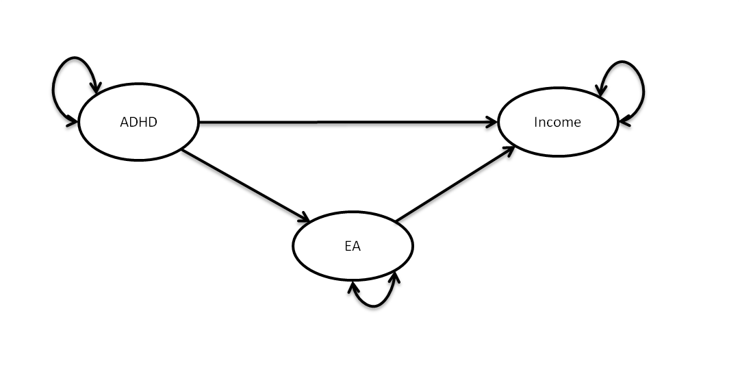
I include a path diagram of the model we are going to fit to awnser our question:
Using GenomicSEM we can test this hypothesis. In order to do so we need the summary statistics for GWAS of all three traits.
I got summary data for a GWAS of ADHD here (I use the 2017 GWAS): https://www.med.unc.edu/pgc/results-and-downloads
I got summary statistics for the GWAS of EA here (I use Okbay et al 2016): https://www.thessgac.org/data
I got summary data for the GWAS on income here: http://www.ccace.ed.ac.uk/node/335
I manually renamed the P-value column in the income summary statistics file "P" because it contained a character which R doesn't like
I launch R and load all the packages I need, I assume OpenMx and devtoolsand semPlot are installed and just need to be loaded.
library("devtools")
install_github("MichelNivard/GenomicSEM")
require(GenomicSEM)
require(OpenMx)
require(semPlot)
I then munge (the term used to describe cleaing and preparation of sumstats) the raw summary statistic files I have downloaded. The argument: "w_hm3.snplist" makes sure we only retain high quality SNPs which were avaialble in HapMap3. This requires the presence of the file "w_hm3.snplist" in the working directory, the file is available here: https://data.broadinstitute.org/alkesgroup/LDSCORE/w_hm3.snplist.bz2
I then use the function ldsc to read the munged files and compute the genetic covariance matrix S, and its parameter variance covariance matrix V (the covariance and variances of the entires in the covariance matrix). This is done automatically, and the results are stored in the R object Data.
munge(c("adhd_jul2017", "EduYears_Main.txt", "Hill2016_UKB_Income_summary_results_21112016.txt"), "w_hm3.snplist",trait.names=c("ADHD_2017",  "EduYears_Main.LDSC","Income"), c(55000,328000,112000), info.filter = 0.9, maf.filter = 0.01)


Data <- ldsc(traits =c("ADHD_2017.sumstats.gz","EduYears_Main.LDSC.sumstats.gz","Income.sumstats.gz"),sample.prev = c(.36,NA,NA),population.prev = c(.06,NA,NA),ld ="eur_w_ld_chr/",wld="eur_w_ld_chr/" )
Now I can proceed to define the model I set out to fit, In the model I regress V3 (3th variable to be read into R using ldsc, so income in this case) on both EA (V2) and ADHD (V1), I also regress EA on ADHD. This creates a path form ADHD to income diectly AND a path from ADHD via EA to income. R/LAVAAN users will recognize the formula notation.
#
MediationModel <- 'V3 ~ V1 + V2
V2 ~ V1'
I then fit the structural equation model using the GenomicSEMfunction usermodel.
#run the model using the user defined function
Mediationoutput <-usermodel(Data, estimation = "DWLS", model = MediationModel )

#print the output
Mediationoutput
The ouput I get is:
$modelfit
   chisq df p_chisq AIC CFI        SRMR
df    NA  0      NA  NA   1 1.22729e-11

$results
   lhs op rhs Unstandardized_Estimate Unstandardized_SE Standardized_Est Standardized_SE
1   V3  ~  V1             -0.08367571       0.032756438       -0.1618597      0.06336304
2   V3  ~  V2              0.52512177       0.037541999        0.7224616      0.05165022
3   V2  ~  V1             -0.37496013       0.025606687       -0.5271930      0.03600294
10  V1 ~~  V1              0.22432924       0.014649729        1.0000000      0.06530459
11  V2 ~~  V2              0.08193974       0.005503839        0.7220675      0.04850080
12  V3 ~~  V3              0.01969760       0.004370548        0.3285535      0.07290018
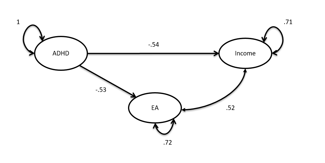
Or in the form of a path model:

Based on these results we would conclude that there is a direct effect of ADHD on income beyond its influence on EA which itself strongly influences income (direct effect of ADHD on income = -.16 se = .06).
To appriciate the magnitude of mediation consider this model, in which there is no mediation, but simply a correlation between EA and income.
DirectModel <- 'V3 ~ V1
V2 ~ V1
V2 ~~ V3'

#run the model using the user defined function
Directoutput <-usermodel(Data, estimation = "DWLS", model = DirectModel )

Directoutput
$modelfit
   chisq df p_chisq AIC CFI         SRMR
df    NA  0      NA  NA   1 2.567592e-09

$results
   lhs op rhs Unstandardized_Estimate Unstandardized_SE Standardized_Est Standardized_SE
1   V3  ~  V1             -0.28057543       0.026892995       -0.5427364      0.05202097
2   V2  ~  V1             -0.37496013       0.025606687       -0.5271930      0.03600294
3   V2 ~~  V3              0.04302834       0.004534992        0.5216661      0.05498124
10  V1 ~~  V1              0.22432924       0.014649729        1.0000000      0.06530459
11  V2 ~~  V2              0.08193974       0.005503839        0.7220675      0.04850080
12  V3 ~~  V3              0.04229272       0.005959712        0.7054372      0.09940724
The model gives a warning, but this is an ignorable warning. It occurs when the user specifies a correlation between observed variables. Internally GenomicSEM makes models to compute the model chi-square of your model, in doing so it adds these covariances which then appear twice in the same model, but are ignored by LAVAAN.
We can visualize this model as a path model:
The two models aren't statistically distinguisable (see also the caveat's listed below) but one can appriciate that the standardized total effect of ADHD on income in this model is larger (effect = -.54, se = 0.05) than the direct effect in the mediation model (-.16, se = 0.06).
some caveats:
-
We assume the causal directions we imply are true. There existstatistically equivalent, but conceptually different, models where the effect of ADHD on EA is reverse, or any number of different configurations. We cannot stiatistically distinguish between these models. Theory should guide you choices, and the estimated parameters, and implied causal directions, should be considered suspect in the absence of commpeling other lines of evidence to support the choice you make.
-
The model does not control for confounding by unmeasured variables, perhaps taller people get better chances in both school and on the labor market, an unmodelled effect of height on EA and income would then influence our estimates. This issue could be dealth with by adding height to the model.
-
Because the model is saturated, we should ignore the model fit values.
We can fit the same model using genomicSEM and OpenMx, code to do so is printed below, and yields virtually identical results. More info on combining GenomicSEMand OpenMx is found here
rownames(Data$V) <- c("adhd~~adhd","adhd~~EA","adhd~~Income","EA~~EA","EA~~Income" ,"Income~~Income")
colnames(Data$V) <- rownames(Data$V)
rownames(Data$S) <- c("adhd", "EA","Income")
colnames(Data$S) <- rownames(Data$S)

Data$W <- round(solve(Data$V),6)
Data$Sr <- round(Data$S,6)


dataCov  <-mxData(Data$Sr, numObs = 100, means = NA, type = "acov", acov=Data$W, fullWeight=Data$W)


# variance paths
varPaths     <- mxPath( from=c("adhd","EA","Income"),  arrows=2,
                        free=T,lbound = 0, values = c(1,1,1), labels=c("var_ADHD","res_EA","res_Income") )


# regression weights
regPaths     <- mxPath( from=c("adhd","EA"), to="Income", arrows=1,
                        free=c(T,T), values=0, labels=c("beta1_adhd","beta1_EA") )
regPaths2     <- mxPath( from="adhd", to="EA", arrows=1,
                         free=T, values=0, labels=c("beta2_adhd") )


fitFunction <- mxFitFunctionWLS()
# Specify the model:
multiRegModel <- mxModel("Mediation Path Specification", type="RAM",
                         fitFunction,dataCov, manifestVars=c("adhd","EA","Income"),
                         varPaths, regPaths,regPaths2)


multiRegFit <- mxRun(multiRegModel)


# Obtain a model summary:
summary(multiRegFit)