Yorko/topic8_vw.md Secret

## topic8_vw.md

      
    Raw
  

              topic8_vw.md
            
          
     Topic 8. Vowpal Wabbit: Learning with Gigabytes of Data

This week, we'll cover two reasons for Vowpal Wabbit's exceptional training speed, namely, online learning and hashing trick, in both theory and practice. We will try it out on the competition's data as well as with news, movie reviews, and StackOverflow questions.
Outline


Stochastic gradient descent and online learning

1.1. SGD
1.2. Online approach to learning


Categorical data processing: Label Encoding, One-Hot Encoding, Hashing trick

2.1. Label Encoding
2.2. One-Hot Encoding
2.3. Hashing trick


Vowpal Wabbit

3.1. News. Binary classification
3.2. News. Multiclass classification
3.3. IMDB reviews
3.4. Classifying gigabytes of StackOverflow questions


Useful links

import warnings
warnings.filterwarnings('ignore')
import os
import re
import numpy as np
import pandas as pd
from tqdm import tqdm_notebook
from sklearn.datasets import fetch_20newsgroups, load_files
from sklearn.preprocessing import LabelEncoder, OneHotEncoder
from sklearn.model_selection import train_test_split
from sklearn.linear_model import LogisticRegression
from sklearn.metrics import classification_report, accuracy_score, log_loss
from sklearn.metrics import roc_auc_score, roc_curve, confusion_matrix
from scipy.sparse import csr_matrix
import matplotlib.pyplot as plt
%matplotlib inline
import seaborn as sns
1. Stochastic gradient descent and online learning

1.1. Stochastic gradient descent

Despite the fact that gradient descent is one of the first things learned in machine learning and optimization courses, it is one of its modifications, Stochastic Gradient Descent (SGD), that is hard to top.
Recall that the idea of gradient descent is to minimize some function by making small steps in the direction of the fastest decrease. This method was named due to the following fact from calculus: vector $\nabla f = (\frac{\partial f}{\partial x_1}, \ldots \frac{\partial f}{\partial x_n})^T$ of partial derivatives of the function $f(x) = f(x_1, \ldots x_n)$ points to the direction of the fastest function growth. It means that, by moving in the opposite direction (antigradient), it is possible to decrease the function value with the fastest rate.

Here is a snowboarder (me) in Sheregesh, Russia's most popular winter resort. (I highly recommended it if you like skiing or snowboarding). In addition to advertising the beautiful landscapes, this picture depicts the idea of gradient descent. If you want to ride as fast as possible, you need to choose the path of steepest descent. Calculating antigradients can be seen as evaluating the slope at various spots.
Example
The paired regression problem can be solved with gradient descent. Let us predict one variable using another: height with weight. Assume that these variables are lineary dependent. We will use the SOCR dataset.
PATH_TO_ALL_DATA = '../../data/'
data_demo = pd.read_csv(os.path.join(PATH_TO_ALL_DATA, 'weights_heights.csv'))
plt.scatter(data_demo['Weight'], data_demo['Height']);
plt.xlabel('Weight in lb')
plt.ylabel('Height in inches');

Here we have a vector $x$ of dimension $\ell$ (weight of every person i.e. training sample) and $y$, a vector containing the height of every person in the dataset.
The task is the following: find weights $w_0$ and $w_1$ such that predicting height as $y_i = w_0 + w_1 x_i$ (where $y_i$ is $i$-th height value, $x_i$ is $i$-th weight value) minimizes the squared error (as well as mean squared error since $\frac{1}{\ell}$ doesn't make any difference ):
$$SE(w_0, w_1) = \frac{1}{2}\sum_{i=1}^\ell(y_i - (w_0 + w_1x_{i}))^2 \rightarrow min_{w_0,w_1}$$
We will use gradient descent, utilizing the partial derivatives of $SE(w_0, w_1)$ over weights $w_0$ and $w_1$.
An iterative training procedure is then defined by simple update formulas (we change model weights in small steps, proportional to a small constant $\eta$, towards the antigradient of the function $SE(w_0, w_1)$):
$$\begin{array}{rcl} w_0^{(t+1)} = w_0^{(t)} -\eta \frac{\partial SE}{\partial w_0} |{t} \  w_1^{(t+1)} = w_1^{(t)} -\eta \frac{\partial SE}{\partial w_1} |{t} \end{array}$$
Computing the partial derivatives, we get the following:
$$\begin{array}{rcl} w_0^{(t+1)} = w_0^{(t)} + \eta \sum_{i=1}^{\ell}(y_i - w_0^{(t)} - w_1^{(t)}x_i) \  w_1^{(t+1)} = w_1^{(t)} + \eta \sum_{i=1}^{\ell}(y_i - w_0^{(t)} - w_1^{(t)}x_i)x_i \end{array}$$
This math works quite well as long as the amount of data is large (we will not discuss issues with local minima, saddle points, choosing the learning rate, moments and other stuff –- these topics are covered very thoroughly in the Numeric Computation chapter in "Deep Learning").
There is an issue with batch gradient descent -- the gradient evaluation requires the summation of a number of values for every object from the training set. In other words, the algorithm requires a lot of iterations, and every iteration recomputes weights with formula which contains a sum $\sum_{i=1}^\ell$ over the whole training set. What happens when we have billions of training samples?

Hence the motivation for stochastic gradient descent! Simply put, we throw away the summation sign and update the weights only over single training samples (or a small number of them). In our case, we have the following:
$$\begin{array}{rcl} w_0^{(t+1)} = w_0^{(t)} + \eta (y_i - w_0^{(t)} - w_1^{(t)}x_i) \  w_1^{(t+1)} = w_1^{(t)} + \eta (y_i - w_0^{(t)} - w_1^{(t)}x_i)x_i \end{array}$$
With this approach, there is no guarantee that we will move in best possible direction at every iteration. Therefore, we may need many more iterations, but we get much faster weight updates.
Andrew Ng has a good illustration of this in his machine learning course. Let's take a look.

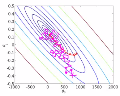
These are the contour plots for some function, and we want to find the global minimum of this function. The red curve shows weight changes (in this picture, $\theta_0$ and $\theta_1$ correspond to our $w_0$ and $w_1$). According to the properties of a gradient, the direction of change at every point is orthogonal to contour plots. With stochastic gradient descent, weights are changing in a less predictible manner, and it even may seem that some steps are wrong by leading away from minima; however, both procedures converge to the same solution.
1.2. Online approach to learning

Stochastic gradient descent gives us practical guidance for training both classifiers and regressors with large amounts of data up to hundreds of GBs (depending on computational resources).
Considering the case of paired regression, we can store the training data set $(X,y)$ in HDD without loading it into RAM (where it simply won't fit), read objects one by one, and update the weights of our model:
$$\begin{array}{rcl} w_0^{(t+1)} = w_0^{(t)} + \eta (y_i - w_0^{(t)} - w_1^{(t)}x_i) \  w_1^{(t+1)} = w_1^{(t)} + \eta (y_i - w_0^{(t)} - w_1^{(t)}x_i)x_i \end{array}$$
After working through the whole training dataset, our loss function (for example, quadratic squared root error in regression or logistic loss in classification) will decrease, but it usually takes dozens of passes over the training set to make the loss small enough.
This approach to learning is called online learning, and this name emerged even before machine learning MOOC-s turned mainstream.
We did not discuss many specifics about SGD here. If you want dive into theory, I highly recommend "Convex Optimization" by Stephen Boyd. Now, we will introduce the Vowpal Wabbit library, which is good for training simple models with huge data sets thanks to stochastic optimization and another trick, feature hashing.
In scikit-learn, classifiers and regressors trained with SGD are named  SGDClassifier and SGDRegressor in sklearn.linear_model. These are nice implementations of SGD, but we'll focus on VW since it is more performant than sklearn's SGD models in many aspects.
2. Categorical feature processing: Label Encoding, One-Hot Encoding, and Hashing trick

2.1. Label Encoding

Many classification and regression algorithms operate in Euclidean or metric space, implying that data is represented with vectors of real numbers. However, in real data, we often have categorical features with discrete values such as yes/no or January/February/.../December. We will see how to process this kind of data, particularly with linear models, and how to deal with many categorial features even when they have many unique values.
Let's explore the UCI bank marketing dataset where most of  features are categorial.
df = pd.read_csv(os.path.join(PATH_TO_ALL_DATA, 'bank_train.csv'))
labels = pd.read_csv(os.path.join(PATH_TO_ALL_DATA,
                                  'bank_train_target.csv'), header=None)

df.head()


      age
      job
      marital
      education
      default
      housing
      loan
      contact
      month
      day_of_week
      duration
      campaign
      pdays
      previous
      poutcome
      emp.var.rate
      cons.price.idx
      cons.conf.idx
      euribor3m
      nr.employed
    
  
      0
      26
      student
      single
      high.school
      no
      no
      no
      telephone
      jun
      mon
      901
      1
      999
      0
      nonexistent
      1.4
      94.465
      -41.8
      4.961
      5228.1
    
    
      1
      46
      admin.
      married
      university.degree
      no
      yes
      no
      cellular
      aug
      tue
      208
      2
      999
      0
      nonexistent
      1.4
      93.444
      -36.1
      4.963
      5228.1
    
    
      2
      49
      blue-collar
      married
      basic.4y
      unknown
      yes
      yes
      telephone
      jun
      tue
      131
      5
      999
      0
      nonexistent
      1.4
      94.465
      -41.8
      4.864
      5228.1
    
    
      3
      31
      technician
      married
      university.degree
      no
      no
      no
      cellular
      jul
      tue
      404
      1
      999
      0
      nonexistent
      -2.9
      92.469
      -33.6
      1.044
      5076.2
    
    
      4
      42
      housemaid
      married
      university.degree
      no
      yes
      no
      telephone
      nov
      mon
      85
      1
      999
      0
      nonexistent
      -0.1
      93.200
      -42.0
      4.191
      5195.8
    
  
We can see that most of features are not represented by numbers. This poses a problem because we cannot use most machine learning methods (at least those implemented in scikit-learn) out-of-the-box.
Let's dive into the "education" feature.
df['education'].value_counts().plot.barh();

The most straightforward solution is to map each value of this feature into a unique number. For example, we can map  university.degree to 0, basic.9y to 1, and so on. You can use sklearn.preprocessing.LabelEncoder to perform this mapping.
label_encoder = LabelEncoder()
The fit method of this class finds all unique values and builds the actual mapping between categories and numbers, and the transform method  converts the categories into numbers. After fit is executed, label_encoder will have the classes_ attribute with all unique values of the feature. Let us count them to make sure the transformation was correct.
mapped_education = pd.Series(label_encoder.fit_transform(df['education']))
mapped_education.value_counts().plot.barh()
print(dict(enumerate(label_encoder.classes_)))
{0: 'basic.4y', 1: 'basic.6y', 2: 'basic.9y', 3: 'high.school', 4: 'illiterate', 5: 'professional.course', 6: 'university.degree', 7: 'unknown'}


df['education'] = mapped_education
df.head()


      age
      job
      marital
      education
      default
      housing
      loan
      contact
      month
      day_of_week
      duration
      campaign
      pdays
      previous
      poutcome
      emp.var.rate
      cons.price.idx
      cons.conf.idx
      euribor3m
      nr.employed
    
  
      0
      26
      student
      single
      3
      no
      no
      no
      telephone
      jun
      mon
      901
      1
      999
      0
      nonexistent
      1.4
      94.465
      -41.8
      4.961
      5228.1
    
    
      1
      46
      admin.
      married
      6
      no
      yes
      no
      cellular
      aug
      tue
      208
      2
      999
      0
      nonexistent
      1.4
      93.444
      -36.1
      4.963
      5228.1
    
    
      2
      49
      blue-collar
      married
      0
      unknown
      yes
      yes
      telephone
      jun
      tue
      131
      5
      999
      0
      nonexistent
      1.4
      94.465
      -41.8
      4.864
      5228.1
    
    
      3
      31
      technician
      married
      6
      no
      no
      no
      cellular
      jul
      tue
      404
      1
      999
      0
      nonexistent
      -2.9
      92.469
      -33.6
      1.044
      5076.2
    
    
      4
      42
      housemaid
      married
      6
      no
      yes
      no
      telephone
      nov
      mon
      85
      1
      999
      0
      nonexistent
      -0.1
      93.200
      -42.0
      4.191
      5195.8
    
  
Let's apply the transformation to other columns of type object.
categorical_columns = df.columns[df.dtypes == 'object'].union(['education'])
for column in categorical_columns:
    df[column] = label_encoder.fit_transform(df[column])
df.head()


      age
      job
      marital
      education
      default
      housing
      loan
      contact
      month
      day_of_week
      duration
      campaign
      pdays
      previous
      poutcome
      emp.var.rate
      cons.price.idx
      cons.conf.idx
      euribor3m
      nr.employed
    
  
      0
      26
      8
      2
      3
      0
      0
      0
      1
      4
      1
      901
      1
      999
      0
      1
      1.4
      94.465
      -41.8
      4.961
      5228.1
    
    
      1
      46
      0
      1
      6
      0
      2
      0
      0
      1
      3
      208
      2
      999
      0
      1
      1.4
      93.444
      -36.1
      4.963
      5228.1
    
    
      2
      49
      1
      1
      0
      1
      2
      2
      1
      4
      3
      131
      5
      999
      0
      1
      1.4
      94.465
      -41.8
      4.864
      5228.1
    
    
      3
      31
      9
      1
      6
      0
      0
      0
      0
      3
      3
      404
      1
      999
      0
      1
      -2.9
      92.469
      -33.6
      1.044
      5076.2
    
    
      4
      42
      3
      1
      6
      0
      2
      0
      1
      7
      1
      85
      1
      999
      0
      1
      -0.1
      93.200
      -42.0
      4.191
      5195.8
    
  
The main issue with this approach is that we have now introduced some relative ordering where it might not exist.
For example, we implicitly introduced algebra over the values of the job feature where we can now substract the job of client #2 from the job of client #1 :
df.loc[1].job - df.loc[2].job
-1.0

Does this operation make any sense? Not really. Let's try to train logisitic regression with this feature transformation.
def logistic_regression_accuracy_on(dataframe, labels):
    features = dataframe.as_matrix()
    train_features, test_features, train_labels, test_labels = \
        train_test_split(features, labels)

    logit = LogisticRegression()
    logit.fit(train_features, train_labels)
    return classification_report(test_labels, logit.predict(test_features))

print(logistic_regression_accuracy_on(df[categorical_columns], labels))
             precision    recall  f1-score   support

          0       0.88      1.00      0.94      6104
          1       0.50      0.00      0.00       795

avg / total       0.84      0.88      0.83      6899

We can see that logistic regression never predicts class 1. In order to use linear models with categorial features, we will use a different approach: One-Hot Encoding.
2.2. One-Hot Encoding

Suppose that some feature can have one of 10 unique values. One-hot encoding creates 10 new features corresponding to these unique values, all of them except one are zeros.
one_hot_example = pd.DataFrame([{i: 0 for i in range(10)}])
one_hot_example.loc[0, 6] = 1
one_hot_example


      0
      1
      2
      3
      4
      5
      6
      7
      8
      9
    
  
      0
      0
      0
      0
      0
      0
      0
      1
      0
      0
      0
    
  
This idea is implemented in the OneHotEncoder class from sklearn.preprocessing. By default OneHotEncoder transforms data into a sparse matrix to save memory space because most of the values are zeroes and because we do not want to take up more RAM. However, in this particular example, we do not encounter such problems, so we are going to use a "dense" matrix representation.
onehot_encoder = OneHotEncoder(sparse=False)
encoded_categorical_columns = pd.DataFrame(onehot_encoder.fit_transform(df[categorical_columns]))
encoded_categorical_columns.head()


      0
      1
      2
      3
      4
      5
      6
      7
      8
      9
      ...
      43
      44
      45
      46
      47
      48
      49
      50
      51
      52
    
  
      0
      0.0
      1.0
      0.0
      1.0
      0.0
      0.0
      0.0
      1.0
      0.0
      0.0
      ...
      0.0
      1.0
      0.0
      0.0
      0.0
      0.0
      0.0
      0.0
      1.0
      0.0
    
    
      1
      1.0
      0.0
      0.0
      0.0
      0.0
      1.0
      0.0
      1.0
      0.0
      0.0
      ...
      0.0
      0.0
      0.0
      0.0
      0.0
      0.0
      0.0
      0.0
      1.0
      0.0
    
    
      2
      0.0
      1.0
      0.0
      0.0
      0.0
      1.0
      0.0
      0.0
      1.0
      0.0
      ...
      0.0
      1.0
      0.0
      0.0
      0.0
      0.0
      0.0
      0.0
      1.0
      0.0
    
    
      3
      1.0
      0.0
      0.0
      0.0
      0.0
      1.0
      0.0
      1.0
      0.0
      0.0
      ...
      1.0
      0.0
      0.0
      0.0
      0.0
      0.0
      0.0
      0.0
      1.0
      0.0
    
    
      4
      0.0
      1.0
      0.0
      1.0
      0.0
      0.0
      0.0
      1.0
      0.0
      0.0
      ...
      0.0
      0.0
      0.0
      0.0
      1.0
      0.0
      0.0
      0.0
      1.0
      0.0
    
  
5 rows × 53 columns

We have 53 columns that correspond to the number of unique values of categorical features in our data set. When transformed with One-Hot Encoding, this data can be used with linear models:
print(logistic_regression_accuracy_on(encoded_categorical_columns, labels))
             precision    recall  f1-score   support

          0       0.90      0.99      0.94      6102
          1       0.67      0.18      0.29       797

avg / total       0.88      0.90      0.87      6899

2.3. Hashing trick

Real data can be volatile, meaning we cannot guarantee that new values of categorial features will not occur. This issue hampers using a trained model on new data. Besides that, LabelEncoder requires preliminary analysis of the whole dataset and storage of constructed mappings in memory, which makes it difficult to work with large datasets.
There is a simple approach to vectorization of categorial data based on hashing and is known as, not-so-surprisingly, the hashing trick.
Hash functions can help us find unique codes for different feature values, for example:
for s in ('university.degree', 'high.school', 'illiterate'):
    print(s, '->', hash(s))
university.degree -> -6241459093488141593
high.school -> 7728198035707179500
illiterate -> -7360093633803373451

We will not use negative values or values of high magnitude, so we restrict the range of values for the hash function:
hash_space = 25
for s in ('university.degree', 'high.school', 'illiterate'):
    print(s, '->', hash(s) % hash_space)
university.degree -> 7
high.school -> 0
illiterate -> 24

Imagine that our data set contains a single (i.e. not married) student, who received a call on Monday. His feature vectors will be created similarly as in the case of One-Hot Encoding but in the space with fixed range for all features:
hashing_example = pd.DataFrame([{i: 0.0 for i in range(hash_space)}])
for s in ('job=student', 'marital=single', 'day_of_week=mon'):
    print(s, '->', hash(s) % hash_space)
    hashing_example.loc[0, hash(s) % hash_space] = 1
hashing_example
job=student -> 20
marital=single -> 23
day_of_week=mon -> 9


      0
      1
      2
      3
      4
      5
      6
      7
      8
      9
      ...
      15
      16
      17
      18
      19
      20
      21
      22
      23
      24
    
  
      0
      0.0
      0.0
      0.0
      0.0
      0.0
      0.0
      0.0
      0.0
      0.0
      1.0
      ...
      0.0
      0.0
      0.0
      0.0
      0.0
      1.0
      0.0
      0.0
      1.0
      0.0
    
  
1 rows × 25 columns

We want to point out that we hash not only feature values but also pairs of feature name + feature value. It is important to do this so that we can distinguish the same values of different features.
assert hash('no') == hash('no')
assert hash('housing=no') != hash('loan=no')
Is it possible to have a collision when using hash codes? Sure, it is possible, but it is a rare case with large enough hashing spaces. Even if collision occurs, regression or classification metrics will not suffer much. In this case, hash collisions work as a form of regularization.

You may be saying "WTF?"; hashing seems counterintuitive. This is true, but these heuristics sometimes are, in fact, the only plausible approach to work with categorial data. Moreover, this technique has proven to just work. As you work more with data, you may see this for yourself.
3. Vowpal Wabbit

Vowpal Wabbit (VW) is one of the most widespread machine learning libraries used in industry. It is prominent for its training speed and support of many training modes, especially for online learning with big and high-dimentional data. This is one of the major merits of the library. Also, with the hashing trick implemented, Vowpal Wabbit is a perfect choice for working with text data.
Shell is the main interface for VW. At least I haven't found the way of installing VW in a Kaggle Kernel (hmm.. Kaggle, what about Docker?), so I've commented out the code in some cells in order to avoid bad outputs.
!vw --help
Num weight bits = 18
learning rate = 0.5
initial_t = 0
power_t = 0.5
using no cache
Reading datafile = 
num sources = 1


VW options:
  --random_seed arg                     seed random number generator
  --ring_size arg                       size of example ring

Update options:
  -l [ --learning_rate ] arg            Set learning rate
  --power_t arg                         t power value
  --decay_learning_rate arg             Set Decay factor for learning_rate 
                                        between passes
  --initial_t arg                       initial t value
  --feature_mask arg                    Use existing regressor to determine 
                                        which parameters may be updated.  If no
                                        initial_regressor given, also used for 
                                        initial weights.

Weight options:
  -i [ --initial_regressor ] arg        Initial regressor(s)
  --initial_weight arg                  Set all weights to an initial value of 
                                        arg.
  --random_weights arg                  make initial weights random
  --normal_weights arg                  make initial weights normal
  --truncated_normal_weights arg        make initial weights truncated normal
  --sparse_weights                      Use a sparse datastructure for weights
  --input_feature_regularizer arg       Per feature regularization input file

Parallelization options:
  --span_server arg                     Location of server for setting up 
                                        spanning tree
  --threads                             Enable multi-threading
  --unique_id arg (=0)                  unique id used for cluster parallel 
                                        jobs
  --total arg (=1)                      total number of nodes used in cluster 
                                        parallel job
  --node arg (=0)                       node number in cluster parallel job

Diagnostic options:
  --version                             Version information
  -a [ --audit ]                        print weights of features
  -P [ --progress ] arg                 Progress update frequency. int: 
                                        additive, float: multiplicative
  --quiet                               Don't output disgnostics and progress 
                                        updates
  -h [ --help ]                         Look here: http://hunch.net/~vw/ and 
                                        click on Tutorial.

Feature options:
  --hash arg                            how to hash the features. Available 
                                        options: strings, all
  --ignore arg                          ignore namespaces beginning with 
                                        character <arg>
  --ignore_linear arg                   ignore namespaces beginning with 
                                        character <arg> for linear terms only
  --keep arg                            keep namespaces beginning with 
                                        character <arg>
  --redefine arg                        redefine namespaces beginning with 
                                        characters of string S as namespace N. 
                                        <arg> shall be in form 'N:=S' where := 
                                        is operator. Empty N or S are treated 
                                        as default namespace. Use ':' as a 
                                        wildcard in S.
  -b [ --bit_precision ] arg            number of bits in the feature table
  --noconstant                          Don't add a constant feature
  -C [ --constant ] arg                 Set initial value of constant
  --ngram arg                           Generate N grams. To generate N grams 
                                        for a single namespace 'foo', arg 
                                        should be fN.
  --skips arg                           Generate skips in N grams. This in 
                                        conjunction with the ngram tag can be 
                                        used to generate generalized 
                                        n-skip-k-gram. To generate n-skips for 
                                        a single namespace 'foo', arg should be
                                        fN.
  --feature_limit arg                   limit to N features. To apply to a 
                                        single namespace 'foo', arg should be 
                                        fN
  --affix arg                           generate prefixes/suffixes of features;
                                        argument '+2a,-3b,+1' means generate 
                                        2-char prefixes for namespace a, 3-char
                                        suffixes for b and 1 char prefixes for 
                                        default namespace
  --spelling arg                        compute spelling features for a give 
                                        namespace (use '_' for default 
                                        namespace)
  --dictionary arg                      read a dictionary for additional 
                                        features (arg either 'x:file' or just 
                                        'file')
  --dictionary_path arg                 look in this directory for 
                                        dictionaries; defaults to current 
                                        directory or env{PATH}
  --interactions arg                    Create feature interactions of any 
                                        level between namespaces.
  --permutations                        Use permutations instead of 
                                        combinations for feature interactions 
                                        of same namespace.
  --leave_duplicate_interactions        Don't remove interactions with 
                                        duplicate combinations of namespaces. 
                                        For ex. this is a duplicate: '-q ab -q 
                                        ba' and a lot more in '-q ::'.
  -q [ --quadratic ] arg                Create and use quadratic features
  --q: arg                              : corresponds to a wildcard for all 
                                        printable characters
  --cubic arg                           Create and use cubic features

Example options:
  -t [ --testonly ]                     Ignore label information and just test
  --holdout_off                         no holdout data in multiple passes
  --holdout_period arg                  holdout period for test only, default 
                                        10
  --holdout_after arg                   holdout after n training examples, 
                                        default off (disables holdout_period)
  --early_terminate arg                 Specify the number of passes tolerated 
                                        when holdout loss doesn't decrease 
                                        before early termination, default is 3
  --passes arg                          Number of Training Passes
  --initial_pass_length arg             initial number of examples per pass
  --examples arg                        number of examples to parse
  --min_prediction arg                  Smallest prediction to output
  --max_prediction arg                  Largest prediction to output

                                        which features have been defined. This 
                                        will lead to smaller cache sizes
  --loss_function arg (=squared)        Specify the loss function to be used, 
                                        uses squared by default. Currently 
                                        available ones are squared, classic, 
                                        hinge, logistic, quantile and poisson.
  --quantile_tau arg (=0.5)             Parameter \tau associated with Quantile
                                        loss. Defaults to 0.5
  --l1 arg                              l_1 lambda
  --l2 arg                              l_2 lambda
  --no_bias_regularization arg          no bias in regularization
  --named_labels arg                    use names for labels (multiclass, etc.)
                                        rather than integers, argument 
                                        specified all possible labels, 
                                        comma-sep, eg "--named_labels 
                                        Noun,Verb,Adj,Punc"

Output model:
  -f [ --final_regressor ] arg          Final regressor
  --readable_model arg                  Output human-readable final regressor 
                                        with numeric features
  --invert_hash arg                     Output human-readable final regressor 
                                        with feature names.  Computationally 
                                        expensive.
  --save_resume                         save extra state so learning can be 
                                        resumed later with new data
  --preserve_performance_counters       reset performance counters when 
                                        warmstarting
  --save_per_pass                       Save the model after every pass over 
                                        data
  --output_feature_regularizer_binary arg
                                        Per feature regularization output file
  --output_feature_regularizer_text arg Per feature regularization output file,
                                        in text
  --id arg                              User supplied ID embedded into the 
                                        final regressor

Output options:
  -p [ --predictions ] arg              File to output predictions to
  -r [ --raw_predictions ] arg          File to output unnormalized predictions
                                        to

Reduction options, use [option] --help for more info:

  --audit_regressor arg                 stores feature names and their 
                                        regressor values. Same dataset must be 
                                        used for both regressor training and 
                                        this mode.

  --search arg                          Use learning to search, 
                                        argument=maximum action id or 0 for LDF

  --replay_c arg                        use experience replay at a specified 
                                        level [b=classification/regression, 
                                        m=multiclass, c=cost sensitive] with 
                                        specified buffer size

  --explore_eval                        Evaluate explore_eval adf policies

  --cbify arg                           Convert multiclass on <k> classes into 
                                        a contextual bandit problem

  --cb_explore_adf                      Online explore-exploit for a contextual
                                        bandit problem with multiline action 
                                        dependent features

  --cb_explore arg                      Online explore-exploit for a <k> action
                                        contextual bandit problem

  --multiworld_test arg                 Evaluate features as a policies

  --cb_adf                              Do Contextual Bandit learning with 
                                        multiline action dependent features.

  --cb arg                              Use contextual bandit learning with <k>
                                        costs

  --csoaa_ldf arg                       Use one-against-all multiclass learning
                                        with label dependent features.  Specify
                                        singleline or multiline.

  --wap_ldf arg                         Use weighted all-pairs multiclass 
                                        learning with label dependent features.
                                          Specify singleline or multiline.

  --interact arg                        Put weights on feature products from 
                                        namespaces <n1> and <n2>

  --csoaa arg                           One-against-all multiclass with <k> 
                                        costs

  --cs_active arg                       Cost-sensitive active learning with <k>
                                        costs

  --multilabel_oaa arg                  One-against-all multilabel with <k> 
                                        labels

  --classweight arg                     importance weight multiplier for class

  --recall_tree arg                     Use online tree for multiclass

  --log_multi arg                       Use online tree for multiclass

  --ect arg                             Error correcting tournament with <k> 
                                        labels

  --boosting arg                        Online boosting with <N> weak learners

  --oaa arg                             One-against-all multiclass with <k> 
                                        labels

  --top arg                             top k recommendation

  --replay_m arg                        use experience replay at a specified 
                                        level [b=classification/regression, 
                                        m=multiclass, c=cost sensitive] with 
                                        specified buffer size

  --binary                              report loss as binary classification on
                                        -1,1

  --bootstrap arg                       k-way bootstrap by online importance 
                                        resampling

  --link arg (=identity)                Specify the link function: identity, 
                                        logistic, glf1 or poisson

  --stage_poly                          use stagewise polynomial feature 
                                        learning

  --lrqfa arg                           use low rank quadratic features with 
                                        field aware weights

  --lrq arg                             use low rank quadratic features

  --autolink arg                        create link function with polynomial d

  --marginal arg                        substitute marginal label estimates for
                                        ids

  --new_mf arg                          rank for reduction-based matrix 
                                        factorization

  --nn arg                              Sigmoidal feedforward network with <k> 
                                        hidden units

confidence options:
  --confidence_after_training           Confidence after training

  --confidence                          Get confidence for binary predictions

  --active_cover                        enable active learning with cover

  --active                              enable active learning

  --replay_b arg                        use experience replay at a specified 
                                        level [b=classification/regression, 
                                        m=multiclass, c=cost sensitive] with 
                                        specified buffer size

  --baseline                            Learn an additive baseline (from 
                                        constant features) and a residual 
                                        separately in regression.

  --OjaNewton                           Online Newton with Oja's Sketch

  --bfgs                                use bfgs optimization

  --conjugate_gradient                  use conjugate gradient based 
                                        optimization

  --lda arg                             Run lda with <int> topics

  --noop                                do no learning

  --print                               print examples

  --rank arg                            rank for matrix factorization.

  --sendto arg                          send examples to <host>

  --svrg                                Streaming Stochastic Variance Reduced 
                                        Gradient

  --ftrl                                FTRL: Follow the Proximal Regularized 
                                        Leader

  --pistol                              FTRL: Parameter-free Stochastic 
                                        Learning

  --ksvm                                kernel svm

Gradient Descent options:
  --sgd                                 use regular stochastic gradient descent
                                        update.
  --adaptive                            use adaptive, individual learning 
                                        rates.
  --adax                                use adaptive learning rates with x^2 
                                        instead of g^2x^2
  --invariant                           use safe/importance aware updates.
  --normalized                          use per feature normalized updates
  --sparse_l2 arg (=0)                  use per feature normalized updates

Input options:
  -d [ --data ] arg                     Example Set
  --daemon                              persistent daemon mode on port 26542
  --foreground                          in persistent daemon mode, do not run 
                                        in the background
  --port arg                            port to listen on; use 0 to pick unused
                                        port
  --num_children arg                    number of children for persistent 
                                        daemon mode
  --pid_file arg                        Write pid file in persistent daemon 
                                        mode
  --port_file arg                       Write port used in persistent daemon 
                                        mode
  -c [ --cache ]                        Use a cache.  The default is 
                                        <data>.cache
  --cache_file arg                      The location(s) of cache_file.
  --json                                Enable JSON parsing.
  --dsjson                              Enable Decision Service JSON parsing.
  -k [ --kill_cache ]                   do not reuse existing cache: create a 
                                        new one always
  --compressed                          use gzip format whenever possible. If a
                                        cache file is being created, this 
                                        option creates a compressed cache file.
                                        A mixture of raw-text & compressed 
                                        inputs are supported with 
                                        autodetection.
  --no_stdin                            do not default to reading from stdin

Vowpal Wabbit reads data from files or from standard input stream (stdin) with the following format:
[Label] [Importance] [Tag]|Namespace Features |Namespace Features ... |Namespace Features
Namespace=String[:Value]
Features=(String[:Value] )*
here [] denotes non-mandatory elements, and (...)* means multiple inputs allowed.

Label is a number. In the case of classification, it is usually 1 and -1; for regression, it is a real float value
Importance is a number. It denotes the sample weight during training. Setting this helps when working with imbalanced data.
Tag is a string without spaces. It is the "name" of the sample that VW saves upon prediction. In order to separate Tag from Importance, it is better to start Tag with the ' character.
Namespace is for creating different feature spaces.
Features are object features inside a given Namespace. Features have weight 1.0 by default, but it can be changed, for example feature:0.1.

The following string matches the VW format:
1 1.0 |Subject WHAT car is this |Organization University of Maryland:0.5 College Park

Let's check the format by running VW with this training sample:
! echo '1 1.0 |Subject WHAT car is this |Organization University of Maryland:0.5 College Park' | vw
Num weight bits = 18
learning rate = 0.5
initial_t = 0
power_t = 0.5
using no cache
Reading datafile = 
num sources = 1
average  since         example        example  current  current  current
loss     last          counter         weight    label  predict features
1.000000 1.000000            1            1.0   1.0000   0.0000       10

finished run
number of examples per pass = 1
passes used = 1
weighted example sum = 1.000000
weighted label sum = 1.000000
average loss = 1.000000
best constant = 1.000000
best constant's loss = 0.000000
total feature number = 10

VW is a wonderful tool for working with text data. We'll illustrate it with the 20newsgroups dataset, which contains letters from 20 different newsletters.
3.1. News. Binary classification.

# load data with sklearn's function 
newsgroups = fetch_20newsgroups(PATH_TO_ALL_DATA)
Downloading 20news dataset. This may take a few minutes.
Downloading dataset from https://ndownloader.figshare.com/files/5975967 (14 MB)

newsgroups['target_names']
['alt.atheism',
 'comp.graphics',
 'comp.os.ms-windows.misc',
 'comp.sys.ibm.pc.hardware',
 'comp.sys.mac.hardware',
 'comp.windows.x',
 'misc.forsale',
 'rec.autos',
 'rec.motorcycles',
 'rec.sport.baseball',
 'rec.sport.hockey',
 'sci.crypt',
 'sci.electronics',
 'sci.med',
 'sci.space',
 'soc.religion.christian',
 'talk.politics.guns',
 'talk.politics.mideast',
 'talk.politics.misc',
 'talk.religion.misc']

Lets look at the first document in this collection:
text = newsgroups['data'][0]
target = newsgroups['target_names'][newsgroups['target'][0]]

print('-----')
print(target)
print('-----')
print(text.strip())
print('----')
-----
rec.autos
-----
From: lerxst@wam.umd.edu (where's my thing)
Subject: WHAT car is this!?
Nntp-Posting-Host: rac3.wam.umd.edu
Organization: University of Maryland, College Park
Lines: 15

 I was wondering if anyone out there could enlighten me on this car I saw
the other day. It was a 2-door sports car, looked to be from the late 60s/
early 70s. It was called a Bricklin. The doors were really small. In addition,
the front bumper was separate from the rest of the body. This is 
all I know. If anyone can tellme a model name, engine specs, years
of production, where this car is made, history, or whatever info you
have on this funky looking car, please e-mail.

Thanks,
- IL
   ---- brought to you by your neighborhood Lerxst ----
----

Now we convert the data into something Vowpal Wabbit can understand. We will throw away words shorter than 3 symbols. Here, we will skip some important NLP stages such as stemming and lemmatization; however, we will later see that VW solves the problem even without these steps.
def to_vw_format(document, label=None):
    return str(label or '') + ' |text ' + ' '.join(re.findall('\w{3,}', document.lower())) + '\n'

to_vw_format(text, 1 if target == 'rec.autos' else -1)
'1 |text from lerxst wam umd edu where thing subject what car this nntp posting host rac3 wam umd edu organization university maryland college park lines was wondering anyone out there could enlighten this car saw the other day was door sports car looked from the late 60s early 70s was called bricklin the doors were really small addition the front bumper was separate from the rest the body this all know anyone can tellme model name engine specs years production where this car made history whatever info you have this funky looking car please mail thanks brought you your neighborhood lerxst\n'

We split the dataset into train and test and write these into separate files. We will consider a document as positive if it corresponds to rec.autos. Thus, we are constructing a model which distinguishes articles about cars from other topics:
all_documents = newsgroups['data']
all_targets = [1 if newsgroups['target_names'][target] == 'rec.autos' 
               else -1 for target in newsgroups['target']]
train_documents, test_documents, train_labels, test_labels = \
    train_test_split(all_documents, all_targets, random_state=7)
    
with open(os.path.join(PATH_TO_ALL_DATA, '20news_train.vw'), 'w') as vw_train_data:
    for text, target in zip(train_documents, train_labels):
        vw_train_data.write(to_vw_format(text, target))
with open(os.path.join(PATH_TO_ALL_DATA, '20news_test.vw'), 'w') as vw_test_data:
    for text in test_documents:
        vw_test_data.write(to_vw_format(text))
Now, we pass the created training file to Vowpal Wabbit. We solve the classification problem with a hinge loss function (linear SVM). The trained model will be saved in the 20news_model.vw file:
!vw -d $PATH_TO_ALL_DATA/20news_train.vw \
 --loss_function hinge -f $PATH_TO_ALL_DATA/20news_model.vw
final_regressor = ../../data//20news_model.vw
Num weight bits = 18
learning rate = 0.5
initial_t = 0
power_t = 0.5
using no cache
Reading datafile = ../../data//20news_train.vw
num sources = 1
average  since         example        example  current  current  current
loss     last          counter         weight    label  predict features
1.000000 1.000000            1            1.0  -1.0000   0.0000      157
0.911276 0.822551            2            2.0  -1.0000  -0.1774      159
0.605793 0.300311            4            4.0  -1.0000  -0.3994       92
0.419594 0.233394            8            8.0  -1.0000  -0.8167      129
0.313998 0.208402           16           16.0  -1.0000  -0.6509      108
0.196014 0.078029           32           32.0  -1.0000  -1.0000      115
0.183158 0.170302           64           64.0  -1.0000  -0.7072      114
0.261046 0.338935          128          128.0   1.0000  -0.7900      110
0.262910 0.264774          256          256.0  -1.0000  -0.6425       44
0.216663 0.170415          512          512.0  -1.0000  -1.0000      160
0.176710 0.136757         1024         1024.0  -1.0000  -1.0000      194
0.134541 0.092371         2048         2048.0  -1.0000  -1.0000      438
0.104403 0.074266         4096         4096.0  -1.0000  -1.0000      644
0.081329 0.058255         8192         8192.0  -1.0000  -1.0000      174

finished run
number of examples per pass = 8485
passes used = 1
weighted example sum = 8485.000000
weighted label sum = -7555.000000
average loss = 0.079837
best constant = -1.000000
best constant's loss = 0.109605
total feature number = 2048932

VW prints a lot of interesting info while training (one can supress it with the --quiet parameter). You can see documentation of the diagnostic output on GitHub. Note how average loss drops while training. For loss computation, VW uses samples it has never seen before, so this measure is usually accurate. Now, we apply our trained model to the test set, saving predictions into a file with the -p flag:
!vw -i $PATH_TO_ALL_DATA/20news_model.vw -t -d $PATH_TO_ALL_DATA/20news_test.vw \
-p $PATH_TO_ALL_DATA/20news_test_predictions.txt
only testing
predictions = ../../data//20news_test_predictions.txt
Num weight bits = 18
learning rate = 0.5
initial_t = 0
power_t = 0.5
using no cache
Reading datafile = ../../data//20news_test.vw
num sources = 1
average  since         example        example  current  current  current
loss     last          counter         weight    label  predict features
    n.a.     n.a.            1            1.0  unknown   1.0000      349
    n.a.     n.a.            2            2.0  unknown  -1.0000       50
    n.a.     n.a.            4            4.0  unknown  -1.0000      251
    n.a.     n.a.            8            8.0  unknown  -1.0000      237
    n.a.     n.a.           16           16.0  unknown  -0.8978      106
    n.a.     n.a.           32           32.0  unknown  -1.0000      964
    n.a.     n.a.           64           64.0  unknown  -1.0000      261
    n.a.     n.a.          128          128.0  unknown   0.4621       82
    n.a.     n.a.          256          256.0  unknown  -1.0000      186
    n.a.     n.a.          512          512.0  unknown  -1.0000      162
    n.a.     n.a.         1024         1024.0  unknown  -1.0000      283
    n.a.     n.a.         2048         2048.0  unknown  -1.0000      104

finished run
number of examples per pass = 2829
passes used = 1
weighted example sum = 2829.000000
weighted label sum = 0.000000
average loss = n.a.
total feature number = 642215

Now we load our predictions, compute AUC, and plot the ROC curve:
with open(os.path.join(PATH_TO_ALL_DATA, '20news_test_predictions.txt')) as pred_file:
    test_prediction = [float(label) 
                             for label in pred_file.readlines()]

auc = roc_auc_score(test_labels, test_prediction)
roc_curve = roc_curve(test_labels, test_prediction)

with plt.xkcd():
    plt.plot(roc_curve[0], roc_curve[1]);
    plt.plot([0,1], [0,1])
    plt.xlabel('FPR'); plt.ylabel('TPR'); plt.title('test AUC = %f' % (auc)); plt.axis([-0.05,1.05,-0.05,1.05]);

The AUC value we get shows that we have achieved high classification quality.
3.2. News. Multiclass classification

We will use the same news dataset, but, this time, we will solve a multiclass classification problem. Vowpal Wabbit is a little picky – it wants labels starting from 1 till K, where K – is the number of classes in the classification task (20 in our case). So we will use LabelEncoder and add 1 afterwards (recall that LabelEncoder maps labels into range from 0 to K-1).
all_documents = newsgroups['data']
topic_encoder = LabelEncoder()
all_targets_mult = topic_encoder.fit_transform(newsgroups['target']) + 1
The data is the same, but we have changed the labels, train_labels_mult and test_labels_mult, into label vectors from 1 to 20.
train_documents, test_documents, train_labels_mult, test_labels_mult = \
    train_test_split(all_documents, all_targets_mult, random_state=7)
    
with open(os.path.join(PATH_TO_ALL_DATA, '20news_train_mult.vw'), 'w') as vw_train_data:
    for text, target in zip(train_documents, train_labels_mult):
        vw_train_data.write(to_vw_format(text, target))
with open(os.path.join(PATH_TO_ALL_DATA, '20news_test_mult.vw'), 'w') as vw_test_data:
    for text in test_documents:
        vw_test_data.write(to_vw_format(text))
We train Vowpal Wabbit in multiclass classification mode, passing the oaa parameter("one against all") with the number of classes. Also, let's see what parameters our model quality is dependent on (more info can be found in the official Vowpal Wabbit tutorial):

learning rate (-l, 0.5 default) – rate of weight change on every step
learning rate decay (--power_t, 0.5 default) – it is proven in practice, that, if the learning rate drops with the number of steps in stochastic gradient descent, we approach the minimum loss better
loss function (--loss_function) – the entire training algorithm depends on it. See docs for loss functions
Regularization (-l1) – note that VW  calculates regularization for every object. That is why we usually set regularization values to about $10^{-20}.$


Additionally, we can try automatic Vowpal Wabbit parameter tuning with Hyperopt.
%%time
!vw --oaa 20 $PATH_TO_ALL_DATA/20news_train_mult.vw -f $PATH_TO_ALL_DATA/20news_model_mult.vw \
--loss_function=hinge
final_regressor = ../../data//20news_model_mult.vw
Num weight bits = 18
learning rate = 0.5
initial_t = 0
power_t = 0.5
using no cache
Reading datafile = ../../data//20news_train_mult.vw
num sources = 1
average  since         example        example  current  current  current
loss     last          counter         weight    label  predict features
1.000000 1.000000            1            1.0       15        1      157
1.000000 1.000000            2            2.0        2       15      159
1.000000 1.000000            4            4.0       15       10       92
1.000000 1.000000            8            8.0       16       15      129
1.000000 1.000000           16           16.0       13       12      108
0.937500 0.875000           32           32.0        2        9      115
0.906250 0.875000           64           64.0       16       16      114
0.867188 0.828125          128          128.0        8        4      110
0.816406 0.765625          256          256.0        7       15       44
0.646484 0.476562          512          512.0       13        9      160
0.502930 0.359375         1024         1024.0        3        4      194
0.388672 0.274414         2048         2048.0        1        1      438
0.300293 0.211914         4096         4096.0       11       11      644
0.225098 0.149902         8192         8192.0        5        5      174

finished run
number of examples per pass = 8485
passes used = 1
weighted example sum = 8485.000000
weighted label sum = 0.000000
average loss = 0.222392
total feature number = 2048932
CPU times: user 10.2 ms, sys: 11.7 ms, total: 21.9 ms
Wall time: 396 ms

%%time
!vw -i $PATH_TO_ALL_DATA/20news_model_mult.vw -t -d $PATH_TO_ALL_DATA/20news_test_mult.vw \
-p $PATH_TO_ALL_DATA/20news_test_predictions_mult.txt
only testing
predictions = ../../data//20news_test_predictions_mult.txt
Num weight bits = 18
learning rate = 0.5
initial_t = 0
power_t = 0.5
using no cache
Reading datafile = ../../data//20news_test_mult.vw
num sources = 1
average  since         example        example  current  current  current
loss     last          counter         weight    label  predict features
    n.a.     n.a.            1            1.0  unknown        8      349
    n.a.     n.a.            2            2.0  unknown        6       50
    n.a.     n.a.            4            4.0  unknown       18      251
    n.a.     n.a.            8            8.0  unknown       18      237
    n.a.     n.a.           16           16.0  unknown        4      106
    n.a.     n.a.           32           32.0  unknown       15      964
    n.a.     n.a.           64           64.0  unknown        4      261
    n.a.     n.a.          128          128.0  unknown        8       82
    n.a.     n.a.          256          256.0  unknown       10      186
    n.a.     n.a.          512          512.0  unknown        1      162
    n.a.     n.a.         1024         1024.0  unknown       11      283
    n.a.     n.a.         2048         2048.0  unknown       14      104

finished run
number of examples per pass = 2829
passes used = 1
weighted example sum = 2829.000000
weighted label sum = 0.000000
average loss = n.a.
total feature number = 642215
CPU times: user 5.29 ms, sys: 9.01 ms, total: 14.3 ms
Wall time: 182 ms

with open(os.path.join(PATH_TO_ALL_DATA, '20news_test_predictions_mult.txt')) as pred_file:
    test_prediction_mult = [float(label) for label in pred_file.readlines()]
accuracy_score(test_labels_mult, test_prediction_mult)
0.8734535171438671

Here is how often the model misclassifies atheism with other topics:
M = confusion_matrix(test_labels_mult, test_prediction_mult)
for i in np.where(M[0,:] > 0)[0][1:]:
    print(newsgroups['target_names'][i], M[0,i])
rec.autos 1
rec.sport.baseball 1
sci.med 1
soc.religion.christian 3
talk.religion.misc 5

3.3. IMDB movie reviews

In this part we will do binary classification of IMDB (International Movie DataBase) movie reviews. We will see how fast Vowpal Wabbit performs.
Using the load_files function from sklearn.datasets, we load the movie reviews here. If you want to reproduce the results, please download the archive, unzip it, and set the path to imdb_reviews (it already contains train and test subdirectories). Unpacking can take several minutes as there are 100k files. Both train and test sets hold 12.5k good and bad movie reviews. First, we split the texts and labels.
import pickle
# change this for your path to imdb_reviews
path_to_movies = os.path.expanduser('/Users/y.kashnitsky/Documents/Machine_learning/datasets/imdb_reviews')
reviews_train = load_files(os.path.join(path_to_movies, 'train'))
text_train, y_train = reviews_train.data, reviews_train.target
print("Number of documents in training data: %d" % len(text_train))
print(np.bincount(y_train))
Number of documents in training data: 25000
[12500 12500]

Do the same for the test set.
reviews_test = load_files(os.path.join(path_to_movies, 'test'))
text_test, y_test = reviews_test.data, reviews_train.target
print("Number of documents in test data: %d" % len(text_test))
print(np.bincount(y_test))
Number of documents in test data: 25000
[12500 12500]

Take a look at examples of reviews and their corresponding labels.
text_train[0]
b"Zero Day leads you to think, even re-think why two boys/young men would do what they did - commit mutual suicide via slaughtering their classmates. It captures what must be beyond a bizarre mode of being for two humans who have decided to withdraw from common civility in order to define their own/mutual world via coupled destruction.<br /><br />It is not a perfect movie but given what money/time the filmmaker and actors had - it is a remarkable product. In terms of explaining the motives and actions of the two young suicide/murderers it is better than 'Elephant' - in terms of being a film that gets under our 'rationalistic' skin it is a far, far better film than almost anything you are likely to see. <br /><br />Flawed but honest with a terrible honesty."

y_train[0] # good review
1

text_train[1]
b'Words can\'t describe how bad this movie is. I can\'t explain it by writing only. You have too see it for yourself to get at grip of how horrible a movie really can be. Not that I recommend you to do that. There are so many clich\xc3\xa9s, mistakes (and all other negative things you can imagine) here that will just make you cry. To start with the technical first, there are a LOT of mistakes regarding the airplane. I won\'t list them here, but just mention the coloring of the plane. They didn\'t even manage to show an airliner in the colors of a fictional airline, but instead used a 747 painted in the original Boeing livery. Very bad. The plot is stupid and has been done many times before, only much, much better. There are so many ridiculous moments here that i lost count of it really early. Also, I was on the bad guys\' side all the time in the movie, because the good guys were so stupid. "Executive Decision" should without a doubt be you\'re choice over this one, even the "Turbulence"-movies are better. In fact, every other movie in the world is better than this one.'

y_train[1] # bad review
0

to_vw_format(str(text_train[1]), 1 if y_train[0] == 1 else -1)
'1 |text words can describe how bad this movie can explain writing only you have too see for yourself get grip how horrible movie really can not that recommend you that there are many clich xc3 xa9s mistakes and all other negative things you can imagine here that will just make you cry start with the technical first there are lot mistakes regarding the airplane won list them here but just mention the coloring the plane they didn even manage show airliner the colors fictional airline but instead used 747 painted the original boeing livery very bad the plot stupid and has been done many times before only much much better there are many ridiculous moments here that lost count really early also was the bad guys side all the time the movie because the good guys were stupid executive decision should without doubt you choice over this one even the turbulence movies are better fact every other movie the world better than this one\n'

Now, we prepare training (movie_reviews_train.vw), validation (movie_reviews_valid.vw), and test (movie_reviews_test.vw) sets for Vowpal Wabbit. We will use 70% for training, 30% for the hold-out set.
train_share = int(0.7 * len(text_train))
train, valid = text_train[:train_share], text_train[train_share:]
train_labels, valid_labels = y_train[:train_share], y_train[train_share:]
len(train_labels), len(valid_labels)
(17500, 7500)

with open(os.path.join(PATH_TO_ALL_DATA, 'movie_reviews_train.vw'), 'w') as vw_train_data:
    for text, target in zip(train, train_labels):
        vw_train_data.write(to_vw_format(str(text), 1 if target == 1 else -1))
with open(os.path.join(PATH_TO_ALL_DATA, 'movie_reviews_valid.vw'), 'w') as vw_train_data:
    for text, target in zip(valid, valid_labels):
        vw_train_data.write(to_vw_format(str(text), 1 if target == 1 else -1))
with open(os.path.join(PATH_TO_ALL_DATA, 'movie_reviews_test.vw'), 'w') as vw_test_data:
    for text in text_test:
        vw_test_data.write(to_vw_format(str(text)))
!head -2 $PATH_TO_ALL_DATA/movie_reviews_train.vw
1 |text zero day leads you think even think why two boys young men would what they did commit mutual suicide via slaughtering their classmates captures what must beyond bizarre mode being for two humans who have decided withdraw from common civility order define their own mutual world via coupled destruction not perfect movie but given what money time the filmmaker and actors had remarkable product terms explaining the motives and actions the two young suicide murderers better than elephant terms being film that gets under our rationalistic skin far far better film than almost anything you are likely see flawed but honest with terrible honesty
-1 |text words can describe how bad this movie can explain writing only you have too see for yourself get grip how horrible movie really can not that recommend you that there are many clich xc3 xa9s mistakes and all other negative things you can imagine here that will just make you cry start with the technical first there are lot mistakes regarding the airplane won list them here but just mention the coloring the plane they didn even manage show airliner the colors fictional airline but instead used 747 painted the original boeing livery very bad the plot stupid and has been done many times before only much much better there are many ridiculous moments here that lost count really early also was the bad guys side all the time the movie because the good guys were stupid executive decision should without doubt you choice over this one even the turbulence movies are better fact every other movie the world better than this one

!head -2 $PATH_TO_ALL_DATA/movie_reviews_valid.vw
1 |text matter life and death what can you really say that would properly justice the genius and beauty this film powell and pressburger visual imagination knows bounds every frame filled with fantastically bold compositions the switches between the bold colours the real world the stark black and white heaven ingenious showing visually just how much more vibrant life the final court scene also fantastic the judge and jury descend the stairway heaven hold court over peter david niven operation all the performances are spot roger livesey being standout and the romantic energy the film beautiful never has there been more romantic film than this there has haven seen matter life and death all about the power love and just how important life and jack cardiff cinematography reason enough watch the film alone the way lights kim hunter face makes her all the more beautiful what genius can make simple things such game table tennis look exciting and the sound design also impeccable the way the sound mutes vital points was decision way ahead its time this true classic that can restore anyone faith cinema under appreciated its initial release and today audiences but one all time favourites which why give this film word beautiful
1 |text while this was better movie than 101 dalmations live action not animated version think still fell little short what disney could was well filmed the music was more suited the action and the effects were better done compared 101 the acting was perhaps better but then the human characters were given far more appropriate roles this sequel and glenn close really not missed the first movie she makes shine her poor lackey and the overzealous furrier sidekicks are wonderful characters play off and they add the spectacle disney has given this great family film with little objectionable material and yet remains fun and interesting for adults and children alike bound classic many disney films are here hoping the third will even better still because you know they probably want make one

!head -2 $PATH_TO_ALL_DATA/movie_reviews_test.vw
 |text don hate heather graham because she beautiful hate her because she fun watch this movie like the hip clothing and funky surroundings the actors this flick work well together casey affleck hysterical and heather graham literally lights the screen the minor characters goran visnjic sigh and patricia velazquez are talented they are gorgeous congratulations miramax director lisa krueger
 |text don know how this movie has received many positive comments one can call artistic and beautifully filmed but those things don make for the empty plot that was filled with sexual innuendos wish had not wasted time watch this movie rather than being biographical was poor excuse for promoting strange and lewd behavior was just another hollywood attempt convince that that kind life normal and from the very beginning asked self what was the point this movie and continued watching hoping that would change and was quite disappointed that continued the same vein glad did not spend the money see this theater

Now, launch Vowpal Wabbit with the following arguments:

-d, path to training set (corresponding .vw file)
--loss_function – hinge (feel free to experiment here)
-f – path to the output file (which can also be in the .vw format)

!vw -d $PATH_TO_ALL_DATA/movie_reviews_train.vw --loss_function hinge \
-f $PATH_TO_ALL_DATA/movie_reviews_model.vw --quiet
Next, make the hold-out prediction with the following VW arguments:

-i –path to the trained model (.vw file)
-t -d – path to hold-out set (.vw file)
-p – path to a txt-file where the predictions will be stored

!vw -i $PATH_TO_ALL_DATA/movie_reviews_model.vw -t \
-d $PATH_TO_ALL_DATA/movie_reviews_valid.vw -p $PATH_TO_ALL_DATA/movie_valid_pred.txt --quiet
Read the predictions from the text file and estimate the accuracy and ROC AUC. Note that VW prints probability estimates of the +1 class. These estimates are distributed from  -1 to 1, so we can convert these into binary answers, assuming that positive values belong to class 1.
with open(os.path.join(PATH_TO_ALL_DATA, 'movie_valid_pred.txt')) as pred_file:
    valid_prediction = [float(label) 
                             for label in pred_file.readlines()]
print("Accuracy: {}".format(round(accuracy_score(valid_labels, 
               [int(pred_prob > 0) for pred_prob in valid_prediction]), 3)))
print("AUC: {}".format(round(roc_auc_score(valid_labels, valid_prediction), 3)))
Accuracy: 0.885
AUC: 0.942

Again, do the same for the test set.
!vw -i $PATH_TO_ALL_DATA/movie_reviews_model.vw -t \
-d $PATH_TO_ALL_DATA/movie_reviews_test.vw \
-p $PATH_TO_ALL_DATA/movie_test_pred.txt --quiet
with open(os.path.join(PATH_TO_ALL_DATA, 'movie_test_pred.txt')) as pred_file:
    test_prediction = [float(label) 
                             for label in pred_file.readlines()]
print("Accuracy: {}".format(round(accuracy_score(y_test, 
               [int(pred_prob > 0) for pred_prob in test_prediction]), 3)))
print("AUC: {}".format(round(roc_auc_score(y_test, test_prediction), 3)))
Accuracy: 0.88
AUC: 0.94

Let's try to achieve a higher accuracy by incorporating bigrams.
!vw -d $PATH_TO_ALL_DATA/movie_reviews_train.vw \
--loss_function hinge --ngram 2 -f $PATH_TO_ALL_DATA/movie_reviews_model2.vw --quiet
!vw -i$PATH_TO_ALL_DATA/movie_reviews_model2.vw -t -d $PATH_TO_ALL_DATA/movie_reviews_valid.vw \
-p $PATH_TO_ALL_DATA/movie_valid_pred2.txt --quiet
with open(os.path.join(PATH_TO_ALL_DATA, 'movie_valid_pred2.txt')) as pred_file:
    valid_prediction = [float(label) 
                             for label in pred_file.readlines()]
print("Accuracy: {}".format(round(accuracy_score(valid_labels, 
               [int(pred_prob > 0) for pred_prob in valid_prediction]), 3)))
print("AUC: {}".format(round(roc_auc_score(valid_labels, valid_prediction), 3)))
Accuracy: 0.894
AUC: 0.954

!vw -i $PATH_TO_ALL_DATA/movie_reviews_model2.vw -t -d $PATH_TO_ALL_DATA/movie_reviews_test.vw \
-p $PATH_TO_ALL_DATA/movie_test_pred2.txt --quiet
with open(os.path.join(PATH_TO_ALL_DATA, 'movie_test_pred2.txt')) as pred_file:
    test_prediction2 = [float(label) 
                             for label in pred_file.readlines()]
print("Accuracy: {}".format(round(accuracy_score(y_test, 
               [int(pred_prob > 0) for pred_prob in test_prediction2]), 3)))
print("AUC: {}".format(round(roc_auc_score(y_test, test_prediction2), 3)))
Accuracy: 0.888
AUC: 0.952

Adding bigrams really helped improve our model!
3.4. Classifying gigabytes of StackOverflow questions

Now, let's see Vowpal Wabbit work on large datasets. There is a 10GB dataset of StackOverflow questions here; the processed version can be found here. The original dataset is comprised of 10 million questions; each question can have several tags. The data is quite clean, so don't call it "Big Data", even in a pub. :)

We chose only 10 tags: 'javascript', 'java', 'python', 'ruby', 'php', 'c++', 'c#', 'go', 'scala' and 'swift'. Let's solve the 10-class classification problem: we want to predict a tag corresponding to one of these 10 popular programming languages given only the text of the question.
# change the path to data
PATH_TO_STACKOVERFLOW_DATA = '/Users/y.kashnitsky/Documents/stackoverflow_10mln/'
Print the first 3 lines from a sample of the dataset.
!head -3 $PATH_TO_STACKOVERFLOW_DATA/stackoverflow_train.vw
1 | i ve got some code in window scroll that checks if an element is visible then triggers another function however only the first section of code is firing both bits of code work in and of themselves if i swap their order whichever is on top fires correctly my code is as follows fn isonscreen function use strict var win window viewport top win scrolltop left win scrollleft bounds this offset viewport right viewport left + win width viewport bottom viewport top + win height bounds right bounds left + this outerwidth bounds bottom bounds top + this outerheight return viewport right lt bounds left viewport left gt bounds right viewport bottom lt bounds top viewport top gt bounds bottom window scroll function use strict var load_more_results ajax load_more_results isonscreen if load_more_results true loadmoreresults var load_more_staff ajax load_more_staff isonscreen if load_more_staff true loadmorestaff what am i doing wrong can you only fire one event from window scroll i assume not
4 | redefining some constant in ruby ex foo bar generates the warning already initialized constant i m trying to write a sort of reallyconstants module where this code should have this behaviour reallyconstants define_constant foo bar gt sets the constant reallyconstants foo to bar reallyconstants foo gt bar reallyconstants foo foobar gt this should raise an exception that is constant redefinition should generate an exception is that possible
1 | in my form panel i added a checkbox setting stateful true stateid loginpanelremeberme then before sending form i save state calling this savestate on the panel all other componenets save their state and whe i reload the page they recall the previous state but checkbox alway start in unchecked state is there any way to force save value

After selecting our 10 tags, we have a 4.7G dataset that we divide into train and test.
!du -hs $PATH_TO_STACKOVERFLOW_DATA/stackoverflow_*.vw
4,7G	/Users/y.kashnitsky/Documents/stackoverflow_10mln//stackoverflow_10mln.vw
1,6G	/Users/y.kashnitsky/Documents/stackoverflow_10mln//stackoverflow_test.vw
3,1G	/Users/y.kashnitsky/Documents/stackoverflow_10mln//stackoverflow_train.vw

We will process the training set (3.1 GiB) with Vowpal Wabbit and the following arguments:

-oaa 10 – for multiclass classification with 10 classes
-d – path to data
-f – path to output file of the trained model
-b 28 – we will use 28 bits for hashing, resulting in a $2^{28}$-sized feature space
fix random seed for reproducibility

%%time
!vw --oaa 10 -d $PATH_TO_STACKOVERFLOW_DATA/stackoverflow_train.vw \
-f vw_model1_10mln.vw -b 28 --random_seed 17 --quiet
CPU times: user 559 ms, sys: 171 ms, total: 730 ms
Wall time: 38.5 s

%%time
!vw -t -i vw_model1_10mln.vw -d $PATH_TO_STACKOVERFLOW_DATA/stackoverflow_test.vw \
-p vw_test_pred.csv --random_seed 17 --quiet
CPU times: user 322 ms, sys: 97.4 ms, total: 420 ms
Wall time: 22.8 s

vw_pred = np.loadtxt(os.path.join(PATH_TO_STACKOVERFLOW_DATA, 'vw_test_pred.csv'))
test_labels = np.loadtxt(os.path.join(PATH_TO_STACKOVERFLOW_DATA, 'stackoverflow_test_labels.txt'))
accuracy_score(test_labels, vw_pred)
0.91728604842865913

The model has trained itself and made predictions in less than a minute (check it, these results are reported for a MacBook Pro, mid 2015, 2.2 GHz Intel Core i7, 16GB RAM). Its accuracy is almost 92%. All of this without a Hadoop cluster! :) Impressive, isn't it?
4. Useful links


Official VW documentation on Github
"Numeric Computation" Chapter of the Deep Learning book
"Convex Optimization" by Stephen Boyd
"Command-line Tools can be 235x Faster than your Hadoop Cluster" post
Benchmarking various ML algorithms on Criteo 1TB dataset on GitHub
VW on FastML.com
	age	job	marital	education	default	housing	loan	contact	month	day_of_week	duration	campaign	pdays	poutcome	emp.var.rate	cons.price.idx	cons.conf.idx	euribor3m	nr.employed
0	26	student	single	high.school	no	no	no	telephone	jun	mon	901	1	999	nonexistent	1.4	94.465	-41.8	4.961	5228.1
1	46	admin.	married	university.degree	no	yes	no	cellular	aug	tue	208	2	999	nonexistent	1.4	93.444	-36.1	4.963	5228.1
2	49	blue-collar	married	basic.4y	unknown	yes	yes	telephone	jun	tue	131	5	999	nonexistent	1.4	94.465	-41.8	4.864	5228.1
3	31	technician	married	university.degree	no	no	no	cellular	jul	tue	404	1	999	nonexistent	-2.9	92.469	-33.6	1.044	5076.2
4	42	housemaid	married	university.degree	no	yes	no	telephone	nov	mon	85	1	999	nonexistent	-0.1	93.200	-42.0	4.191	5195.8
	0	1	3	5	7	8	...	43	44	47	51
0	0.0	1.0	1.0	0.0	1.0	0.0	...	0.0	1.0	0.0	1.0
1	1.0	0.0	0.0	1.0	1.0	0.0	...	0.0	0.0	0.0	1.0
2	0.0	1.0	0.0	1.0	0.0	1.0	...	0.0	1.0	0.0	1.0
3	1.0	0.0	0.0	1.0	1.0	0.0	...	1.0	0.0	0.0	1.0
4	0.0	1.0	1.0	0.0	1.0	0.0	...	0.0	0.0	1.0	1.0