Skip to content

Instantly share code, notes, and snippets.

Created December 31, 2014 18:07
Show Gist options
  • Star 0 You must be signed in to star a gist
  • Fork 4 You must be signed in to fork a gist
  • Save anonymous/fca8450673410b009228 to your computer and use it in GitHub Desktop.
Save anonymous/fca8450673410b009228 to your computer and use it in GitHub Desktop.
Project READMEs - 3D Reconstruction with Computer Vision

Project 1: Panorama stitching

Due: 23 Sept 2014, 11:59pm

In this project, you'll write software that stitches multiple images of a scene together into a panorama automatically. A panorama is a composite image that has a wider field of view than a single image, and can combine images taken at different times for interesting effects.

Your image stitcher will, at a minimum, do the following:

  • locate corresponding points between a pair of images
  • use the corresponding points to fit a homography (2D projective transform) that maps one image into the space of the other
  • use the homography to warp images into a common target frame, resizing and cropping as necessary
  • composite several images in a common frame into a panorama

While I encourage you to make use of OpenCV's powerful libraries, for this project you must not use any of the functions in the stitcher package (although you're welcome to read its documentation and code for inspiration).

Find a homography between two images (40 points + up to 20 bonus points)

A homography is a 2D projective transformation, represented by a 3x3 matrix, that maps points in one image frame to another, assuming both images are captured with an ideal pinhole camera.

Feature matching

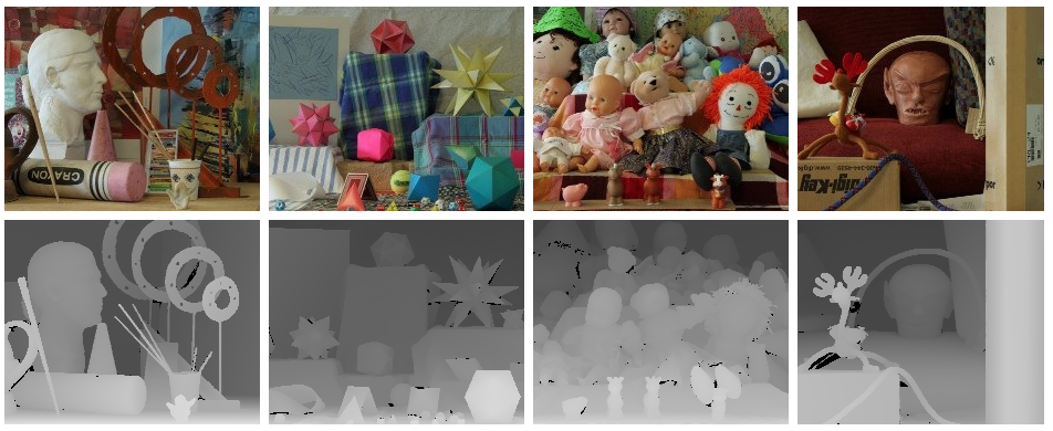
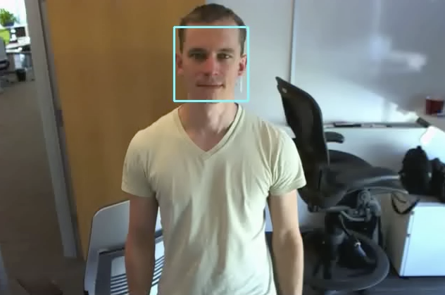
To establish a homography between two images, you'll first need to find a set of correspondences between them. One common way of doing this is to identify "interest points" or "key points" in both images, summarize their appearances using descriptors, and then establish matches between these "features" (interest points combined with their descriptors) by choosing features with similar descriptors from each image.

You're welcome to establish correspondences any way you like. I would recommend you consider extracting keypoints and descriptors using the cv2.SIFT interface to compute interest points and descriptors, and using one of the descriptor matchers OpenCV provides under a common interface.

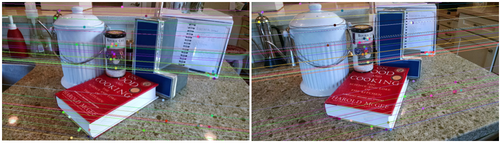
You'll probably find it useful to visualize the matched features between two images to see how many of them look correct. It's a good bet that you'll have some incorrect matches, or "outliers". You can experiment with different feature extraction and matching techniques to try to reduce the number of outliers. The fewer there are, the better the fit of your homography will be, although you'll never be able to eliminate all of them.

Fitting the homography

Once you've established correspondences between two images, you'll use them to find a "best" homography mapping one image into the frame of another. Again, you're welcome to do this any way you like, but I suggest you consider looking at cv2.findHomography, which can compute the least-squares-best-fit homography given a set of corresponding points. It also offers robustified computation using RANSAC or the Least-Median methods. You'll likely need to tweak the robustifiers' parameters to get the best results.

Evaluating success

The unit tests include test_homography, which will evaluate the difference between your computed homography and a "ground truth" known homography. If your homography is close enough to ground truth for this test to pass, you'll receive full credit. You'll lose points as the accuracy of your homography declines.

Bonus credit

I will evaluate your homography computation with a broad selection of input images and ground-truth homographies, and measure the distribution of error norms. The most accurate implementation in class will recieve 20 bonus points. The second most accurate will receive 16, the third 12, the fourth 8, and the fifth 4.

I expect you'll need to delve into the details of feature matching and robust fitting to achieve the highest possible accuracy.

Image warping (20 points)

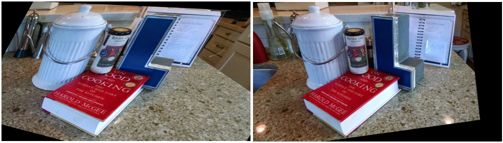
Once you've found homographies mapping all images into a common frame, you'll need to actually warp them according to these homographys before you can composite them together. This process is also referred to as "image rectification." A good place to start is [cv.warpPerspective](http://docs.opencv.org/modules/imgproc/doc/geometric_transformations.html#void warpPerspective(InputArray src, OutputArray dst, InputArray M, Size dsize, int flags, int borderMode, const Scalar& borderValue)), but be aware that out-of-the-box, it may map images outside the target image coordinates.

In addition to warping the image, you should add an alpha channel so that pixels not covered by the warped input image are "clear" before compositing. For a full specification of the expected behavior, see the function comment for warp_image() and its corresponding unit tests.

Image mosaicing (20 points)

Composite your images together into a mosaic to form the final output panorama. You don't need to blend the images together (although you can for extra credit; see below), but there should be no occlusion of one image by another except where at least one image has valid warped pixels.

Write up and results (20 points)

Capture at least one set of three or more images using any camera you like (your phone's camera will probably do fine) and stitch the images together into a panorama with your implementation. Add the source images, the panorama, and a script that can regenerate the pano from your implementation into the my_panos folder. Include a write_up.txt or write_up.pdf describing how to run your script, and any interesting information about your solution you'd like to share.

If you want, play around! Try taking a panorama where the same person or object appears multiple times. Try distant and close up scenes to see the effects of parallax on your solution. Place any interesting panos in the my_panos folder and I'll share the results with the class.

Extra credit (maximum of 50 points)

There's a lot more to explore in the world of homographies and panorama stitching. Implement as many of the below as you like for extra credit. Be sure to include code for the extra credit as part of your check-in. Also, please add a PDF write-up describing which extra credit you implemented called extra_credit.pdf in the project_1 directory so we can see your results.

10 points: Panorama of a planar scene

Instead of taking all of your panoramas from the same spot, create a panorama by moving linearly along in front of a planar scene. Report your results and the challenges of taking such a pano.

10 points: Image cut-out compositing

Identify a known planar surface in an image and composite a planar image onto it. You can use this technique to add graffiti or a picture of your self to an image of a building.

10-20 points: Blending

Implement some form of alpha blending between overlapping images. Some possibilities include feathering, pyramid blending, or multi-band blending. The more sophisticated and higher-quality blending you use, the more points you'll earn.

20 points: Spherical stitching

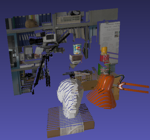
Instead of mapping all of your images into a single perspective frame, map them into spherical coordinates (this will require a guess of the focal length of the camera). This will allow you to create any spherical projection of your panorama, like the lovely "little planet":

Globe panorama03.jpg

Or the equirectangular projection:

Such panos will look better if they cover as much of the sphere as possible.

Logistics

You will work on this project in randomly assigned groups of three. All group members should have identical submissions in each of their private repositories by the project due date. We will select one group member's repository, clone it, and use it to compute the grade for all group members.

If the group chooses to turn in a project N days late, each individual in the group will lose N of their remaining late days for the semester. If one or more students have no more late days left, they'll lose credit without affecting the other group members' grades.

Project 2: Stereo

Due: 14 Oct 2014, 11:59pm

Code reviews due: 17 Oct 2014, 11:59pm

Final code revisions due: 21 Oct 2014, 11:59pm

In this project, you'll reconstruct a 3D scene from stereo image pairs.

At a minimum, your stereo reconstruction implementation will:

  • identify epipolar geometry of a stereo pair
  • compute a fundamental matrix relating epipolar geometry from one image to the other
  • compute homographies to rectify the stereo images so epipolar lines are in corresponding rows
  • compute disparities between rectified stereo images
  • convert disparities to a 3D model

Rectify a stereo image pair (30 points)

Epipolar geometry relates two stereo cameras and images by constrainting where corresponding points lie in their images. Most stereo algorithms rely on epipolar lines lying in corresponding image rows of a stereo pair. The process of converting a pair of input images to a new pair where epipolar lines lie on corresponding image rows is called image rectification.

Feature matching

Just as when we were matching images for panorama stitching, the first thing we need to do to compute epipolar geometry from a pair of images is to establish some correspondences between the images. One common way of doing this is to identify "interest points" or "key points" in both images, summarize their appearances using descriptors, and then establish matches between these "features" (interest points combined with their descriptors) by choosing features with similar descriptors from each image.

You're welcome to establish correspondences any way you like. I would recommend you consider extracting keypoints and descriptors using the cv2.SIFT interface to compute interest points and descriptors, and using one of the descriptor matchers OpenCV provides under a common interface.

Computing the fundamental matrix

The fundamental matrix maps points in one stereo image to epipolar lines in the other. It can be computed using corresponding points in two images recovered in the feature matching stage. In particular, cv2.findFundamentalMat() implements just this approach. Here's an example of epipolar lines mapped using the fundamental matrix between stereo images:

Rectifying the images

Once we know the fundamental matrix, we can compute homographies that warp the images in the pair so that corresponding rows in the two images are epipolar lines. See cv2.stereoRectifyUncalibrated().

You may find it helpful to crop the images to just the mutually overlapping regions of the rectified images, to avoid computation where there are no corresponding pixels present in one or the other image.

Disparity computation (20 points)

Once we have a rectified stereo pair, the next step is to compute disparities between correponding pixels. There are many strategies and algorithms to do this, and most have plenty of parameters to tune. You may want to start by looking at StereoBM and StereoSGBM which are part of the OpenCV library.

To get the best results from disparity computation, you'll need to carefully consider each parameter and its effect on the disparity image output. There is a lot of "art" to tuning disparity computation, so you'll probably want to look at many inputs, not just the one used in the unit test. For a bunch of example inputs, most with ground-truth disparities, see the Middlebury Stereo Datasets page.

Point cloud conversion (10 points)

Disparity can be converted to depth if we know the focal length of the camera. Although we can't know this focal length exactly for an uncalibrated camera like our cell phone, we can take a guess and see the results in 3D.

Implement a function that converts a disparity image to a PLY point cloud, given a focal length. For an example of one way to do this, see the stereo_match.py example from the OpenCV source code, although beware that their Q projection matrix is buggy. You will want a projection matrix similar to:

[ 1  0             0   image_width / 2 ]
[ 0  1             0  image_height / 2 ]
[ 0  0  focal_length                 0 ]
[ 0  0             0                 1 ]

You can view your PLY point clouds in Meshlab.

Results (20 points)

Capture at least one stereo pair of images using any camera you like (your phone's camera will probably do fine) and create a disparity image and 3D point cloud using your implemenation. Add the source images, the disparity image, the point cloud, and a script that can regenerate the outputs from your implementation into the my_stereo folder. Include a README.txt or README.md (Markdown format) explaining how to regenerate your panos.

You'll find that it can be tough to make a good stereo scene. Try to move the camera deliberately to capture a clear change of viewpoint, but not too much, so there is still a lot of shared surfaces visible on both images. Include textured objects in your scene so that disparity computation algorithms have a better chance of success. Play around and see what works best.

Code quality and review (20 points)

Above and beyond just passing the pep8 style checker, you should strive to write readable, modular, well-factored code. As in project 1, each group will review three other groups code, and then receive ratings on the quality of their review. You'll receive up to 10 points for the quality of your groups review. After you revise your code in response to review, we'll go over your final code and rate it's quality for up to another 10 points. Hint: the style and comments of OpenCV tutorials is not a model you should emulate :)

Extra credit (maximum of 50 points)

There's a lot more to stereo than the minimum specified above. Complete any of the additional work below for extra credit.

Be sure to include code for the extra credit as part of your check-in. Also, please add a PDF write-up describing which extra credit you implemented including your results called extra_credit.pdf in the project_2 directory so we can see your results.

Implement your own disparity computation (20 points)

Implement any algorithm for computing disparity from a rectified stereo pair. There is an excellent overview of many popular algorithms here.

Prove that your implementation works by using it to produce a disparity image from a rectified stereo pair.

Implement multi-view stereo reconstruction of 3D models (30 points)

Multi-view stereo uses not just 2 but N images of a scene or object to extract a more complete 3D model of the scene. See this site for an overview of several multi-view stereo methods, as well as example input data sets that you can use to test your implementation.

Prove that your implementation works by using it to produce a 3D model of an object. It's fine to use one of the example inputs, but consider trying to make a 3D model of an interesting object you have lying around!

Logistics

You will work on this project in randomly assigned groups of three. All group members should have identical submissions in each of their private repositories by the project due date. We will select one group member's repository, clone it, and use it to compute the grade for all group members.

If the group chooses to turn in a project N days late, each individual in the group will lose N of their remaining late days for the semester. If one or more students have no more late days left, they'll lose credit without affecting the other group members' grades.

Project 3: Tracking

Due: 4 Nov 2014, 11:59pm

Code reviews due: 7 Nov 2014, 11:59pm

Final code revisions due: 11 Nov 2014, 11:59pm

In this project, you'll track objects in video sequences. There are many effective methods to do this for the problems provided, so unlike previous projects, you will have to choose which particular approach works best for you for each problem case. I suggest a thorough consideration of OpenCV's libraries when designing solutions.

Think back over the different methods for tracking and motion detection discussed in class, including background subtraction, optical flow, sparse feature tracking, and Kalman filtering. You can use any combination of these techniques (and others!) to accomplish your tracking tasks.

Tracking the bounds of a solid-colored ball (50 points)

For this part of the project, you'll track a ball as it moves across different background fields. There are four input videos, ball_{1,2,3,4}.mov. You'll need to track the ball's motion in each video.

Implement four functions, track_ball_{1,2,3,4}(), which track the bounds of the ball in each of the four input videos. It's likely that the implementation of these four functions will share some helper functions, or may just call a single shared implementation, perhaps with different parameters.

Your function will return, for each frame of the video, the (min_x, min_y, max_x, max_y) tuple describing the rectangular bounding box around the ball. The bounds will be compared against the ground truth bounds in test_data/ball_bounds.txt.

Your implementation may not make use of any "ground truth" information about the videos that it does not determine on its own, including the ball's color, initial location, dimensions, or motion.

Tracking the location of a face (30 points)

For this part of the project, you will track a face as it moves in a real video. You will implement a track_face() function that returns output of the same format as your ball tracking functions: a per-frame (min_x, min_y, max_x, max_y) bounding box of the face. You will likely need more sophisticated detection to find a face compared with a ball.

Your implementation may not make sue of any "ground truth" information about the video that it does not determine on its own, including the face's initial location or motion.

Code quality and review (20 points)

Above and beyond just passing the pep8 style checker, you should strive to write readable, modular, well-factored code. As in project 1, each group will review three other groups code, and then receive ratings on the quality of their review. You'll receive up to 5 points for the quality of your groups review. After you revise your code in response to review, we'll go over your final code and rate it's quality for up to another 15 points. Hint: the style and comments of OpenCV tutorials is not a model you should emulate :)

Extra credit (maximum of 50 points)

Tracking is a broad research topic, and we're only scratching the surface with the above tasks. If you like, you can do additional implementation work for extra credit.

Be sure to include code for the extra credit as part of your check-in. Also, please add a PDF write-up describing which extra credit you implemented including your results called extra_credit.pdf in the project_3 directory so we can see your results.

Track multiple pedestrians in a street video (20 points)

Download the ETH annotated pedestrian video dataset from here. Implement multi-object tracking for pedestrians in the video, and compare your results to the labeled ground truth.

Composite a 3D object onto a planar surface in a video (30 points)

Similar to effects in this video, use parallax effects in tracked features in a video to establish a planar surface in the scene, and then composite a 3D model onto the planar surface. Produce a video of the result.

Logistics

You will work on this project in randomly assigned groups of three. All group members should have identical submissions in each of their private repositories by the project due date. We will select one group member's repository, clone it, and use it to compute the grade for all group members.

If the group chooses to turn in a project N days late, each individual in the group will lose N of their remaining late days for the semester. If one or more students have no more late days left, they'll lose credit without affecting the other group members' grades.

Sign up for free to join this conversation on GitHub. Already have an account? Sign in to comment