Created
February 16, 2019 00:03
-
-
Save arvi1000/98eeb8d8a8d5925eb567f0a19c7b2c6b to your computer and use it in GitHub Desktop.
Code to extract data from a pie chart PNG and make a better visual
This file contains bidirectional Unicode text that may be interpreted or compiled differently than what appears below. To review, open the file in an editor that reveals hidden Unicode characters.
Learn more about bidirectional Unicode characters
| library(png) | |
| library(tidyverse) | |
| # 1) read in data ---- | |
| to_matrix <- function(png_file) { | |
| # read PNG to raster (3d array of x * y * color channel) | |
| the_png <- readPNG(png_file) | |
| # extract the rgb values from color channels 1 to 3 (4 is alpha) | |
| out_mat <- sapply(1:3, function(x) round(as.vector(the_png[,,x])*255)) | |
| return(out_mat) | |
| } | |
| pie1 <- to_matrix('~/Desktop/pie1.png') | |
| pie2 <- to_matrix('~/Desktop/pie2.png') | |
| # 2) clustering and data extraction ---- | |
| # whoa we have 25k+ unique colors in here, likely due to artifacts from image | |
| # compression | |
| length(unique(pie1)) | |
| # let's use clustering to group similar colors. since we know exactly how many | |
| # target colors we want, k-means is perfect for this. | |
| # 11 colors from the 1st pie & 9 from the 2nd (includes +1 for the white | |
| # background). we initialize with a large number of centroids | |
| # to get a more stable result | |
| km_fit1 <- kmeans(pie1, centers = 11, nstart = 100) | |
| km_fit2 <- kmeans(pie2, centers = 9, nstart = 90) | |
| # let's extract the key info (color values and pixel counts) | |
| km_to_df <- function(km, label_col) { | |
| data.frame(counts = table(km$cluster), | |
| hex_value = rgb(km$centers, maxColorValue = 255), | |
| label = label_col, | |
| stringsAsFactors = F) | |
| } | |
| plot_dat <- rbind(km_to_df(km_fit1, 'pie 1'), | |
| km_to_df(km_fit2, 'pie 2')) | |
| # drop white, which is just the background | |
| plot_dat <- filter(plot_dat, hex_value != '#FEFEFE') | |
| # 3) plot our results for sanity check ---- | |
| # named vector so we can plot each hex value in the actual color | |
| clr_scale <- unique(plot_dat$hex_value) | |
| names(clr_scale) <- clr_scale | |
| # let's take a look! plot for one pie, dropping the background white | |
| do_plot <- function(which_pie) { | |
| plot_dat %>% | |
| filter(label==which_pie) %>% | |
| ggplot(aes(x=reorder(hex_value, counts.Freq), | |
| y=counts.Freq, | |
| fill=hex_value)) + | |
| geom_col() + | |
| scale_fill_manual(values=clr_scale) + | |
| theme_light() + | |
| theme(legend.position = 'none') + | |
| labs(title = paste0('Pixel Frequency by Color Cluster (', which_pie, ')'), | |
| y = 'count', x = 'cluster centroid') | |
| } | |
| do_plot('pie 1') | |
| do_plot('pie 2') | |
| # 4) data reassembly ---- | |
| # let's add the $/hr labels back by looking up the values in the original pie | |
| # for each color (ordered by frequency) | |
| # it's actually pretty hard to look up the dollar values from the colors, | |
| # bc of the crazy leader lines! | |
| pie1_pay <- c(15,12,10,13,16,13.50,14,15.50,16.50,14.50) | |
| pie2_pay <- c(18,20,17,19,17.50,24,26,22) | |
| plot_dat <- plot_dat %>% | |
| arrange(label, -counts.Freq) %>% | |
| mutate(wage = c(pie1_pay, pie2_pay)) | |
| # now we can finally make our better chart! let's get the percent at each wage, | |
| # and percent making up to that wage | |
| plot_dat <- plot_dat %>% | |
| arrange(wage) %>% | |
| mutate(pct = counts.Freq / sum(plot_dat$counts.Freq), | |
| pct_up_to = cumsum(pct)) | |
| # a bar plot is a safe starter bet | |
| ggplot(plot_dat, aes(x=wage, y=100*pct)) + | |
| geom_col(fill='dodgerblue') + | |
| labs(title='Bike Shop Mechanic Hourly Wage', | |
| subtitle = 'based on survey by @ProBicycleMech, n=200', | |
| y = '% of Respondents', x = '$/hr') + | |
| theme_minimal() + | |
| theme(panel.grid.minor = element_blank()) | |
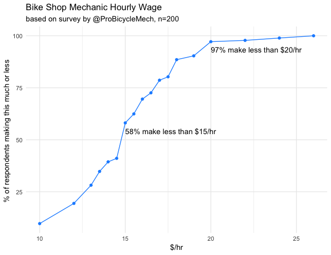
| # but i like a cumulative distribution. maybe less accessible, but | |
| # imo the most informative in this case, esp w some labels | |
| labeler <- function(x, y) { | |
| paste0(round(100*x), '% make less than $', y, '/hr') | |
| } | |
| # the final plot: | |
| ggplot(plot_dat, | |
| aes(x=wage, y=100*pct_up_to)) + | |
| geom_point(color='dodgerblue') + | |
| geom_line(color='dodgerblue') + | |
| geom_text(data = filter(plot_dat, wage %in% c(15, 20)), | |
| aes(label = labeler(pct_up_to, wage)), | |
| vjust = 2, hjust=0) + | |
| labs(title='Bike Shop Mechanic Hourly Wage', | |
| subtitle = 'based on survey by @ProBicycleMech, n=200', | |
| y = '% of respondents making this much or less ', x = '$/hr') + | |
| theme_minimal() + | |
| theme(panel.grid.minor.y = element_blank()) |
Sign up for free
to join this conversation on GitHub.
Already have an account?
Sign in to comment
After: