原文:机器之心
机器之心整理
参与:黄小天、蒋思源
前天,香港科技大学计算机系教授 Sung Kim 在 Google Drive 分享了一个 3 天速成的 TensorFlow 极简入门教程;接着,他在 GitHub 上又分享了一个 3 至 4 日的速成教程,教大家如何使用 PyTorch 进行机器学习/深度学习。Sung Kim 共享了该教程的代码和 PPT 资源,机器之心对其做了扼要介绍。资源链接请见文中。
代码:https://github.com/hunkim/PyTorchZeroToAll
PPT:http://bit.ly/PyTorchZeroAll
百度云盘:https://pan.baidu.com/s/1cpoyXw
PyTorch 开源于今年一月份,它是使用 GPU 和 CPU 优化的深度学习张量库,也是一个 Python 工具包,为目前最流行的深度学习框架之一;它具有两个高阶功能:
带有强大的 GPU 加速的张量计算(类似 NumPy)
构建在基于 tape 的 autograd 系统之上的深度神经网络
因此必要之时你可以再利用 Python 工具包比如 NumPy、SciPy 和 Cython 扩展 PyTorch。PyTorch 目前处于早期的 beta 版,还有待进一步完善与更新。通常来讲,PyTorch 作为库主要包含以下组件:
1. Torch:类似于 NumPy 的张量库,带有强大的 GPU 支持
2. torch.autograd:一个基于 tape 的自动微分库,支持 torch 中的所有的微分张量运算
3. torch.nn:一个专为最大灵活性而设计、与 autograd 深度整合的神经网络库
4. torch.multiprocessing:Python 多运算,但在运算中带有惊人的 torch 张量内存共享。这对数据加载和 Hogwild 训练很有帮助。
5. torch.utils:数据加载器、训练器以及其他便利的实用功能
6. torch.legacy(.nn/.optim):出于后向兼容性原因而从 torch 移植而来的旧代码
人们使用 PyTorch 一般出于两个目的:
代替 NumPy 从而可以使用强大的 GPU
PyTorch 作为深度学习研究平台提供了最大的灵活性与速度
PyTorch 是由若干个资深工程师和研究者共同发起的社区项目,目前主要的维护人员有 Adam Paszke、Sam Gross、Soumith Chintala 和 Gregory Chanan。
PyTorch 课程目录
概览
线性模型
梯度下降
反向传播
PyTorch 线性回归
Logistic 回归
宽&深
数据加载器
Softmax 分类器
CNN
RNN
下面是整个课程的概述:
线性模型
如下为线性模型的基本思想,我们希望能构建一个线性方程拟合现存的数据点。该线性了方程函数将根据数据点与其距离自动调整权重,权重调整的方法即使用优化算法最小化真实数据与预测数据的距离。
以下为该线性模型的实现代码,我们先定义特征 x 与标注 y,然后将预测值与真实值差的平方作为损失函数。随后初始化模型权重并开始前向传播。
import numpy as np
import matplotlib.pyplot as plt
x_data = [1.0, 2.0, 3.0]
y_data = [2.0, 4.0, 6.0]
# our model forward pass
def forward(x):
return x * w
# Loss function
def loss(x, y):
y_pred = forward(x)
return (y_pred - y) * (y_pred - y)
w_list = []
mse_list = []
for w in np.arange(0.0, 4.1, 0.1):
print("w=", w)
l_sum = 0
for x_val, y_val in zip(x_data, y_data):
y_pred_val = forward(x_val)
l = loss(x_val, y_val)
l_sum += l
print("\t", x_val, y_val, y_pred_val, l)
print("NSE=", l_sum / 3)
w_list.append(w)
mse_list.append(l_sum / 3)
plt.plot(w_list, mse_list)
plt.ylabel('Loss')
plt.xlabel('w')
plt.show()
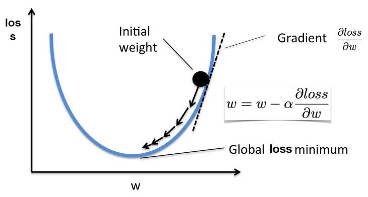
梯度下降
梯度下降在最优化中又称之为最速下降算法,以下为该算法的基本概念。我们可以看到,若我们希望最小化的损失函数为凸函数,那么损失函数对各个权重的偏导数将指向该特征的极小值。如下当初始权重处于损失函数递增部分时,那么一阶梯度即损失函数在该点的斜率,且递增函数的斜率为正,那么当前权重减去一个正数将变小,因此权重将沿递增的反方向移动。同理可得当权重处于递减函数的情况。
如下我们手动实现了简单的梯度下降算法。前面还是先定义模型、损失函数,因为我们已知损失函数的结构,那么就可以手动对其求导以确定梯度函数的结构。得出了权重梯度的表达式后可以将其代入权重更新的循环语句以定义训练。
x_data = [1.0, 2.0, 3.0]
y_data = [2.0, 4.0, 6.0]
w = 1.0 # any random value
# our model forward pass
def forward(x):
return x * w
# Loss function
def loss(x, y):
y_pred = forward(x)
return (y_pred - y) * (y_pred - y)
# compute gradient
def gradient(x, y): # d_loss/d_w
return 2 * x * (x * w - y)
# Before training
print("predict (before training)", 4, forward(4))
# Training loop
for epoch in range(10):
for x_val, y_val in zip(x_data, y_data):
grad = gradient(x_val, y_val)
w = w - 0.01 * grad
print("\tgrad: ", x_val, y_val, grad)
l = loss(x_val, y_val)
print("progress:", epoch, l)
# After training
print("predict (after training)", 4, forward(4))
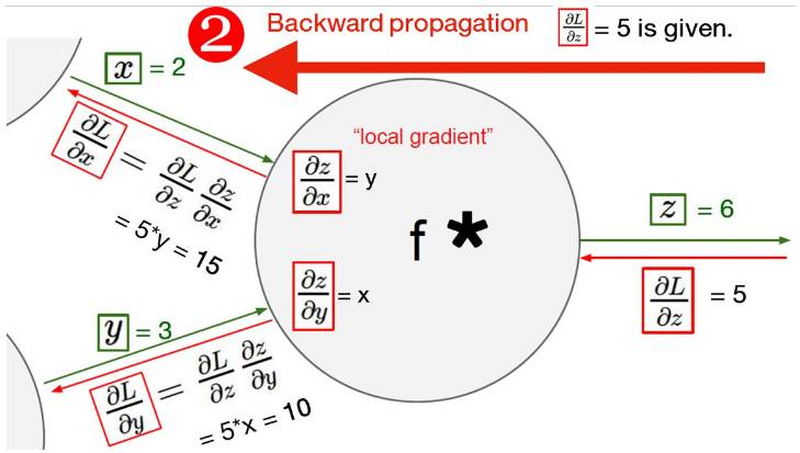
反向传播
下图展示了反向传播算法的链式求导法则与过程。对于反向传播来说,给定权重下,我们先要计算前向传播的结果,然后计算该结果与真实值的距离或误差。随后将该误差沿误差产生的路径反向传播以更新权重,在这个过程中误差会根据求导的链式法则进行分配。
以下代码实现了反向传播算法,我们可以看到在 PyTorch 中反向传播的语句为「loss(x_val, y_val).backward()」,即将损失函数沿反向传播。
import torch
from torch import nn
from torch.autograd import Variable
x_data = [1.0, 2.0, 3.0]
y_data = [2.0, 4.0, 6.0]
w = Variable(torch.Tensor([1.0]), requires_grad=True) # Any random value
# our model forward pass
def forward(x):
return x * w
# Loss function
def loss(x, y):
y_pred = forward(x)
return (y_pred - y) * (y_pred - y)
# Before training
print("predict (before training)", 4, forward(4).data[0])
# Training loop
for epoch in range(10):
for x_val, y_val in zip(x_data, y_data):
l = loss(x_val, y_val)
l.backward()
print("\tgrad: ", x_val, y_val, w.grad.data[0])
w.data = w.data - 0.01 * w.grad.data
# Manually zero the gradients after updating weights
w.grad.data.zero_()
print("progress:", epoch, l.data[0])
# After training
print("predict (after training)", 4, forward(4).data[0])
PyTorch 线性回归
定义数据:
import torch
from torch.autograd import Variable
x_data = Variable(torch.Tensor([[1.0], [2.0], [3.0]]))
y_data = Variable(torch.Tensor([[2.0], [4.0], [6.0]]))
定义模型,在 PyTorch 中,我们可以使用高级 API 来定义相关的模型或层级。如下定义了「torch.nn.Linear(1, 1)」,即一个输入变量和一个输出变量。
class Model(torch.nn.Module):
def __init__(self):
"""
In the constructor we instantiate two nn.Linear module
"""
super(Model, self).__init__()
self.linear = torch.nn.Linear(1, 1) # One in and one out
def forward(self, x):
"""
In the forward function we accept a Variable of input data and we must return
a Variable of output data. We can use Modules defined in the constructor as
well as arbitrary operators on Variables.
"""
y_pred = self.linear(x)
return y_pred
构建损失函数和优化器,构建损失函数也可以直接使用「torch.nn.MSELoss(size_average=False)」调用均方根误差函数。优化器可以使用「torch.optim.SGD()」提到用随机梯度下降,其中我们需要提供优化的目标和学习率等参数。
# Construct our loss function and an Optimizer. The call to model.parameters()
# in the SGD constructor will contain the learnable parameters of the two
# nn.Linear modules which are members of the model.
criterion = torch.nn.MSELoss(size_average=False)
optimizer = torch.optim.SGD(model.parameters(), lr=0.01)
训练模型,执行前向传播计算损失函数,并优化参数:
# Training loop
for epoch in range(500):
# Forward pass: Compute predicted y by passing x to the model
y_pred = model(x_data)
# Compute and print loss
loss = criterion(y_pred, y_data)
print(epoch, loss.data[0])
# Zero gradients, perform a backward pass, and update the weights.
optimizer.zero_grad()
loss.backward()
optimizer.step()
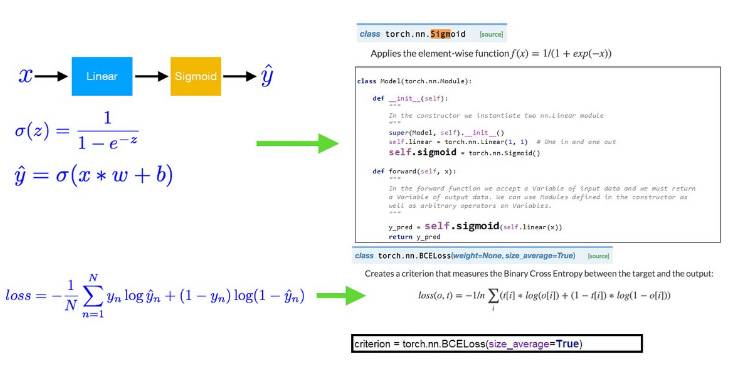
Logistic 回归
以下展示了 Logistic 回归的基本要素和对应代码。Logistic 回归的构建由以下三种函数组成:Sigmoid 函数、目标函数以及损失函数。下图分别给出了三种函数的对应代码。其中 Sigmoid 函数将线性模型演变为 Logistic 回归模型,而损失函数负责创建标准以测量目标与输出之间的二值交叉熵。
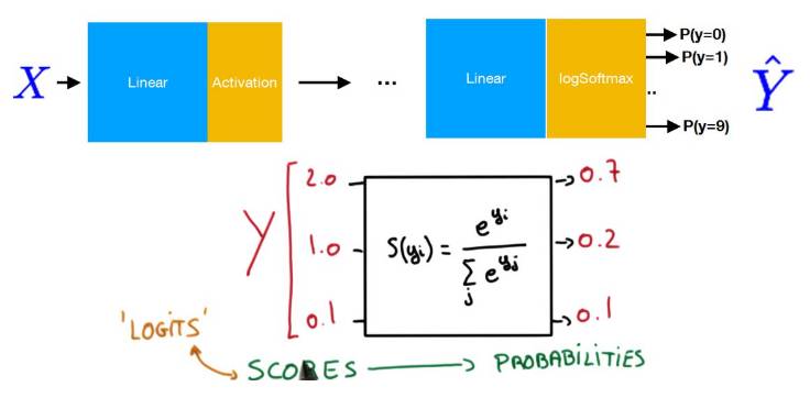
Softmax 分类
以下展示了 Softmax 分类的基本概念,其中最重要的是在最后一层使用了 Softmax 函数。我们可以使用 Softmax 函数将输出值转化为和为 1 的类别概率。
加载数据集与导入数据加载器:
# MNIST Dataset
train_dataset = datasets.MNIST(root='./data/',
train=True,
transform=transforms.ToTensor(),
download=True)
test_dataset = datasets.MNIST(root='./data/',
train=False,
transform=transforms.ToTensor())
# Data Loader (Input Pipeline)
train_loader = torch.utils.data.DataLoader(dataset=train_dataset,
batch_size=batch_size,
shuffle=True)
test_loader = torch.utils.data.DataLoader(dataset=test_dataset,
batch_size=batch_size,
shuffle=False)
定义模型的架构,并选择优化器。如下我们可以了解该 Softmax 分类模型在前面使用了五个全连接层,并在最后一层使用了 Softmax 函数。例如先使用「l1 = nn.Linear(784, 520)」定义全连接的输入结点数与输出结点数,784 为 MNIST 的像素点数,再使用「F.relu(self.l1(x))」定义该全连接的激活函数为 ReLU。
class Net(nn.Module):
def __init__(self):
super(Net, self).__init__()
self.l1 = nn.Linear(784, 520)
self.l2 = nn.Linear(520, 320)
self.l3 = nn.Linear(320, 240)
self.l4 = nn.Linear(240, 120)
self.l5 = nn.Linear(120, 10)
def forward(self, x):
x = x.view(-1, 784) # Flatten the data (n, 1, 28, 28)-> (n, 784)
x = F.relu(self.l1(x))
x = F.relu(self.l2(x))
x = F.relu(self.l3(x))
x = F.relu(self.l4(x))
x = F.relu(self.l5(x))
return F.log_softmax(x)
model = Net()
optimizer = optim.SGD(model.parameters(), lr=0.01, momentum=0.5)
CNN
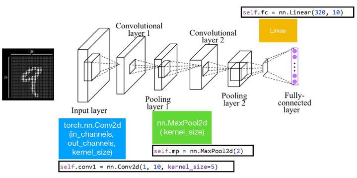
下图展示了一个简单的卷积神经网络,它由输入层、卷积层 1、池化层 1、卷积层 2、池化层 2、全连接层组成。其中卷积层 1、2 是二维的,其输入通道为 1,输出通道为 10,卷积核大小为 5。其中池化层采用的是最大池化运算。
以下是上图简单卷积神经网络的加载数据:
# MNIST Dataset
train_dataset = datasets.MNIST(root='./data/',
train=True,
transform=transforms.ToTensor(),
download=True)
test_dataset = datasets.MNIST(root='./data/',
train=False,
transform=transforms.ToTensor())
# Data Loader (Input Pipeline)
train_loader = torch.utils.data.DataLoader(dataset=train_dataset,
batch_size=batch_size,
shuffle=True)
test_loader = torch.utils.data.DataLoader(dataset=test_dataset,
batch_size=batch_size,
shuffle=False)
以下代码定义了上图卷积神经网络的架构,并定义了优化器。我们同样可以使用高级 API 添加卷积层,例如「nn.Conv2d(1, 10, kernel_size=5)」可以添加卷积核为 5 的卷积层。此外,在卷积层与全连接层之间,我们需要压平张量,这里使用的是「x.view(in_size, -1)」。
class Net(nn.Module):
def __init__(self):
super(Net, self).__init__()
self.conv1 = nn.Conv2d(1, 10, kernel_size=5)
self.conv2 = nn.Conv2d(10, 20, kernel_size=5)
self.mp = nn.MaxPool2d(2)
self.fc = nn.Linear(320, 10)
def forward(self, x):
in_size = x.size(0)
x = F.relu(self.mp(self.conv1(x)))
x = F.relu(self.mp(self.conv2(x)))
x = x.view(in_size, -1) # flatten the tensor
x = self.fc(x)
return F.log_softmax(x)
model = Net()
optimizer = optim.SGD(model.parameters(), lr=0.01, momentum=0.5)
本文为机器之心整理,转载请联系本公众号获得授权。
✄------------------------------------------------
加入机器之心(全职记者/实习生):hr@jiqizhixin.com
投稿或寻求报道:content@jiqizhixin.com
广告&商务合作:bd@jiqizhixin.com