Notes on Business Stats Ch 9.

9.1.md

9.1 Logic of Hypothesis Testing

Hypothesis Testing Steps

1. State Hypothesis

   H₀ - Null Hypothesis H₁ - Alternative Hypothesis

2. Specify Decision Rule

   How to prove the null hypothesis with the evidence

3. Data Collection and Decision Making

   Collect data and use decision rule to reject or not reject hypothesis

4. Take Action Based on Decision

   Do shit with the results.

Type Errors

Type I | a | False Positive - Accepting a hypothesis that is not actually true, aka level of significance Type II | b | False Negative - Not accepting a hypothesis that is actually true

Both have consequences, but false negatives can be a bit more consequential.

Relationship Between a(type I) and b(type II)

Powerful test is a smaller probablity of B. The best way to reduce them together is by increasing sample size, but is not always practical.

9.2.md

9.2 Statistical Hypothesis Testing

u<sub>0</sub> - the benchmark
This isn't from _our sample_, this is derived from a standard or a spec. 
It's how we compare our sample u against this benchmark.

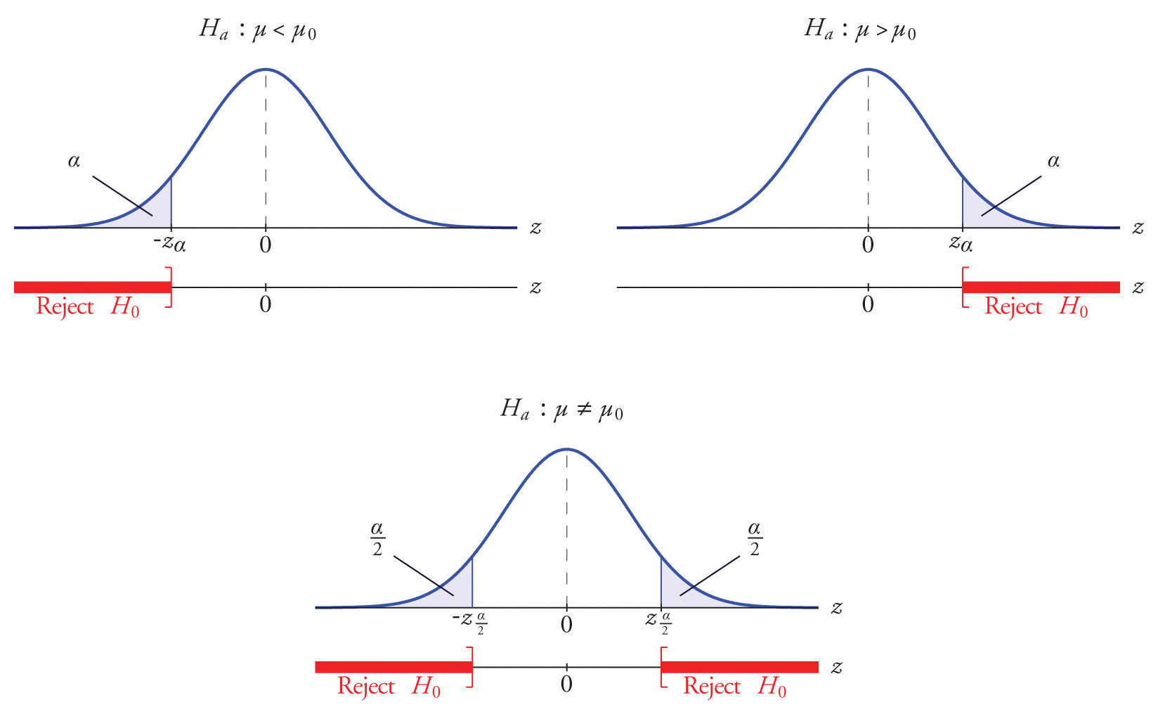
When we determine tailed-test we look at the direction of the inequality points in H₁

• Left-Tailed: u < u₀
• Two-Tailed: u != u₀
• Right-Tailed: u > u₀

Decision Rule

This is the deciding factor of the outcome of our test. Every test is a comparison against the null hypothesis (a "truthy" standard, unless known otherwise) to understanding if an extreme outcome is occuring, causing us to REJECT the hypothesis.

Rejection Region - Area under the curve which represents an extreme outcome
Test Statistics - The difference of the sample statistics and the hypothesized parameter, when it falls in the rejection region it will result in a fail test.

comparison of tailed test

Crtical Value - Basically the bounds of when to reject H₀, or not to (z or t value based on known std).
Decision Rule - Based on step 2, it will define what the critical value is based on our level of significance (a | prob of type I error).

We are looking for a small value of a preferably. For example, in a normal distribution, 95% is a benchmark of a standard level of acceptance, thus we would want less than 5% of a chance for type I errors (false positives, rejecting a true hypothesis) to occur.... a = .05 (.05/2 for each tail if it's a two-tailed test). But if we increase our level of acceptance, 99%, we can only deny our hypothesis if extremes occur within 1%, a = .01.

9.3.md

9.3 Testing a Mean: Known Population Variance

Test Statistic: Z_calc

The z-score is the test statistics if we know u and std, and represents our standardized score for the sample statistics. The z calculated score should be near 0 if the sample mean is close to the true mean of the population.

Critical Value

We compare our calculated z-score to the critical value stated in our hypothesis, this will determine if to reject hypothesis or not. In a two tailed test, we know the risk is split between both tails (a/2).

P-Value Method

Another way that is preferred because you account for the strength in your evidence against the null hypothesis. It's a measure of the chance of the observed sample