cjoy/data-structures-notes.md

## data-structures-notes.md

      
    Raw
  

              data-structures-notes.md
            
          
    ADTs


ADT Interfaces:

Opaque view of a data structure (eg. typedef struct t *T, we don't know struct t)
Function signatures for all operations
Semantics of operations (via documentation, etc)
A contract between ADT and clients


ADT implementations

Concrete defintion of the data structures
Function implementations for all operations


Linked Lists


A sequence of collection of 'nodes' holding value + pointer(s)


No random access


Easy to add, rearrange, remove nodes...


List nodes references other list nodes:

Singly Linked List: next
Doubly Linked List: next prev


Operations

Insertion ~ O(N)
Deletion ~ O(N)
Search ~ O(N)
Intersection ~ O(N+M)


Stacks


LIFO (Last In First Out) data structure


List implementation:

Push: Append node to head of the list ~ O(1)
Pop: Remove and return head ~ O(1)
struct stack {
    struct node *head;
    struct node *tail;
    size_t size;
};

struct node {
    Item item;
    struct node *next;
}


Array Implementation

Allocate an array with a maximum number of elements
Fill items sequentially
Maintain a counter of the number of pushed / popped items (ie. the top)
Push: Increment top and set new top array index to value ~ O(1)
Pop: Decrement top and return the last hightest value
Disadvantage: Fixed size stack (Unless it's a dyanamically growing array)
struct stack {
    int top;
    Item *items;
};


Queues


FIFO (First In First Out) data structure
List Implementation

struct queue {
    struct node *head;
    struct node *tail;
}

struct node {
    Item item;
    struct node *next;
}

Insert: O(N) - without tail pointer in struct, otherwise O(1)
Deletion: O(1)

Analysis


Emperical: executing and measuring


Theoretical: proving and deriving


Factors:

Correctness: returns expected output
Robustness: behaves sensibly for non-valid inputs
Efficiency: returns results reasonably quickly
Clarity: clear code
Consistency: interface is clear & consistent


We will only focus on correctness and efficiency.


Testing (Correctness)


Postel's Robustness Principle: "Be conservative in what you do; be liberal in what you accept from others"


TDD (Test Driven Development): write tests first, then write the function & repeat


Regression testing: Keep a test suite and always run the tests after each update to the program


Black-box testing: checks behaviour using only the interface (ie the ADT interface)


White-box testing: checks internal behaviour (when we can see and test the ADT implementation)


Complexity (Efficency)


Algorithm runtime tends to be a function of input size


Focus on asymptotic worst-case execution time


Take into account all possible input ranges


Cases: Best Case / Average Case / Worst Case


Binary search example:

start at middle for sorted list

is the middle the key? if not continue


if item is less, we search in left range (lo, mid)
otherwise, we search in right range (mid+1, hi)


Best case: O(1) ~ middle value


Worst case:

t(N) = 1 + t(N/2) = log(N) + 1
~ O(log n)


Complexity Classes

O(1)          - Constant - Constant time execution, independant of input size.
O(log n)      - Logarithmic - Some divide-and-conquer algorithms with trivial split/recombine operations.
O(n)          - Linear - Every element of the input has to be processed
O(n log n)    - n-log-n - Divide and conquer algorithms, where split / recombine is proportional to input
O(n^2)        - Quadratic - Compute every input with every other input
O(n^3)        - Cubic - misery
O(n!)         - Factorial - what the...
O(2^n)        - Exponential - nope


O(1) < O(log n) < O(n) < O(n log n) < O (n^2) < O(n^3) < O (n!) < O(2^n)


N^2 Algo ie. when N=1000 takes 1.2seconds, how long for

N=2000      x2      ->   x4         4.8 seconds
N=10,000    x10     ->   x100       120 seconds
N=100,000   x100    ->   x10000     12000 seconds
N=1000000   x1000   ->   x1000000   1200000 seconds


Apply ^2 to how much times number of items increases. Multiply that number with base case.


Tractable: have a polynomial time ('P') algorithm


Intractable: no tractable algorithm exists (usually 'NP')


Non-computable: no algorithm exists


Recursion


Base case (or stopping case): where no recursive call is needed
Recursive case: calls the function on a smaller version of the problem.
Steps:

Solve as if you're not using recursion for basic subset of problem
Use self for solving the rest


eg. n! = (n-1)! x n

f(0)=1 f(1) = 1 else f(n) = n*f(n-1)


Usually iterative and recusrive has same time complexity (ie. arry_max, binary_search)

Trees


Trees are branches data structures of nodes and edges with no cycles.
Each node contains a value
Each node has edges <=k other nodes (k = 2 for binary trees)
Node is parent if it has outgoing edges
Node is child if it has incoming edges
Depth (or height) is the number of edges from the root to that node;
A leaf is a node with no children.
Trees can be viewed as set of nested structures
Values in the left subtree has to be less than the node value
Vice versa for right subtree.
Degenerate: maximal height (n-1)
Balanced: minimal height (log n)

Size: |size(L) - size(R)| < 2
Height: |height(L) - height(R)| < 2


Advantages

Faster search O(log n) - compared with linked lists
Faster inseartion O(log n) - compared with array O(N)


Binary trees


A binary tree with n nodes has a height of at most n-1, if degenerate or least floor(log n) if balanced
Complete binary tree have hieght ceiling(log n).
Insertion: balanced ~ O(log n), degenerate ~ O(n) ie. have to traverse the tree, like a llist
Search / Deletion: balanced ~ O(log n), degenerate O(n)
All nodes in left are less than and vice versa
Structure determined by order of insertion

Tree Traversals


Depth First:

Pre-order traversal (NLR)
In-order traversal (LNR) - visits elements in sorted order - when tree is a BST.
Post-order traversal (LRN)


Breath First:

Level-order traversal: visit node and all its children

ie. Like a BFS, where you use a queue
basically visits each level from left to right
use a queue

void tree_level_order_traversal (Tree t)
{
    if (!t) return;

    Queue q = newQueue(40);
    QueueJoin(q, t);
    while (!QueueIsEmpty(q)) {
        Item n = QueueLeave(q);
        printf("%d ", n->item);
        if (n->left) QueueJoin(q, n->left);
        if (n->right) QueueJoin(q, n->right);
    }

    dropQueue(q);
}


Tree successors (In order)

Case 1: node has right subtree

Find the minimum (left most value) of the right sub tree


Case 2: no right subtree

TODO!! https://www.youtube.com/watch?v=5cPbNCrdotA&list=PL2_aWCzGMAwI3W_JlcBbtYTwiQSsOTa6P&index=38&t=0s


Method 2: Perform an in order traversal, store in array and do a linear search for successor (very inefficient, but works)


Deleting a node

Swap value with left most value from the right subtree (ie. it's successor)
Delete the item
Perform rotations (if required - ie. splay tree)


Priority Queue (Using Heaps)


Process in order of key or priority.
Altered enqueue and dequeue operations
Enqueue: join item with a priority.

FixUp operation has to be done, since we insert node at bottom.


Dequeue: remove item with highest priority Q.

FixDown operation has to be done, since we remove top node, by swapping with last item. Last item may not be ideal canditate for top root.


Heaps


Commonly viewed as trees, implemented using arrays.


Two properties to maintain:

heap order property
complete tree property


Heaps have top-to-bottom  ordering (whereas binary trees have left to right ordering)


Heaps are complete trees!

Every level is filled before adding nodes to the next level
Nodes in given level are filled left-to-right with ni breaks


Arrays are good for heaps

parent(i) = i/2
left_child(i) = 2i
right_child(i) = 2i+1


Inserting:

Add new element at the bottom-most, right-most position (to ensure complete tree property)
Reorganise values along the path to the root (to ensure it maintains heap order)


We call this the heap fixup operation
O(log n)


Deleting is a three-step process:

Swap root value with bottom-most, right-most value (ie. last element of array)
Remove that element
Reorganise values along the path from root (to ensure it maintains heap order)


We call this the heap fix down operation
O(log n)


Graphs


Models relationship between items


A graph G is a set of vertices V and edges E

E := {(v,w) | v,w is an element of V, (v,w) is an element of V X V}
Basically a set of edges [(v,w)]


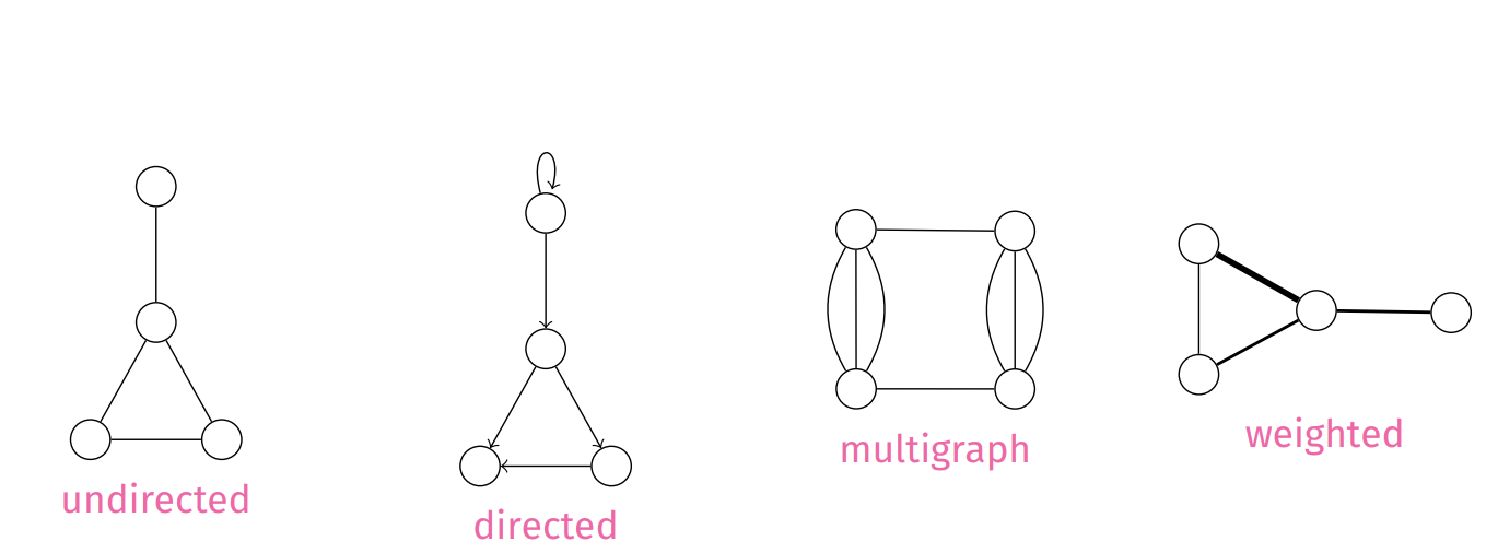
Simple graphs

a set of vertices
a set of undirected edges
no self loops
no parallel edges


Sparcity vs Density

Sparcity ~ less connections between nodes

|E| approaches |V|


Density ~ more connections between nodes

|E| approaches |V|^2


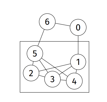
Subgraph: subset of vertices and associate edges


Path: Sequence of connected vertices ie [(v,e) elem 1]


Simple path: no repeating vertices


Cycle: path with start and end vertex as the same.


How to find:

Perform a DFS.
Whilst performing a DFS, if visiting already visited node, then it has a cycle.


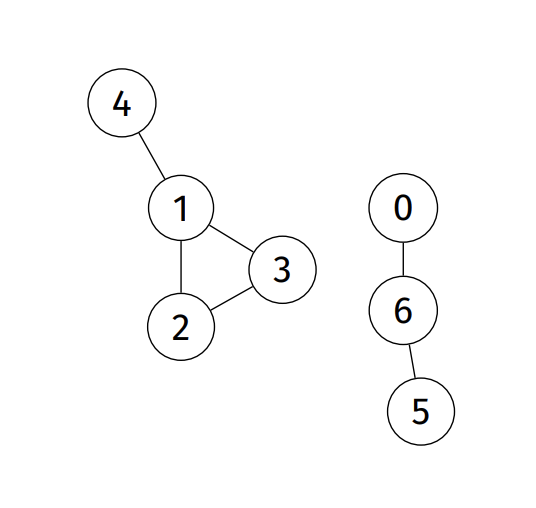
Connected graph: a path exists from every node to every other node


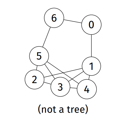
Tree: connected graph with no cycles


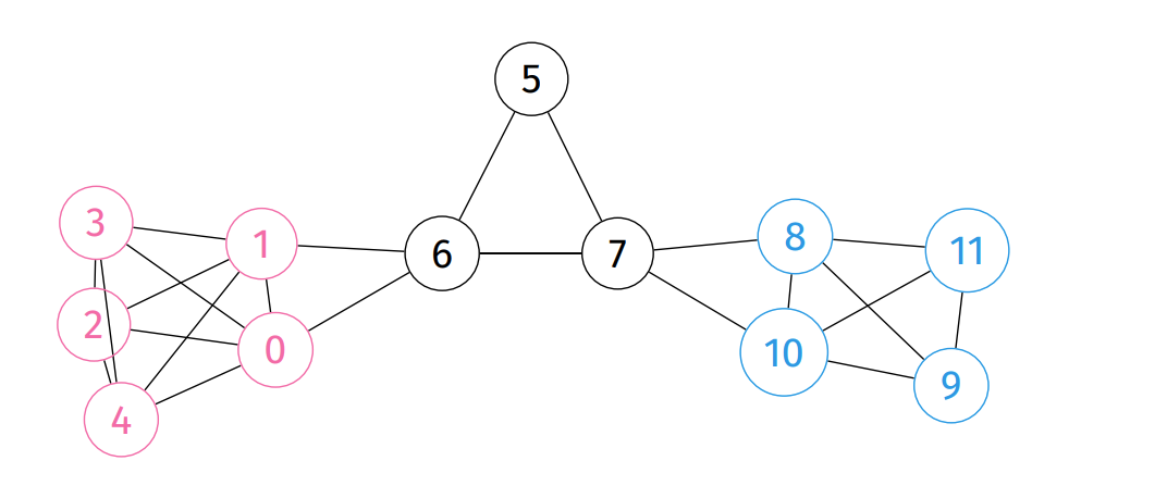
Connected components: a graph that's not connected, consisting of a set of connected components.

ie. maximally connected subgraphs


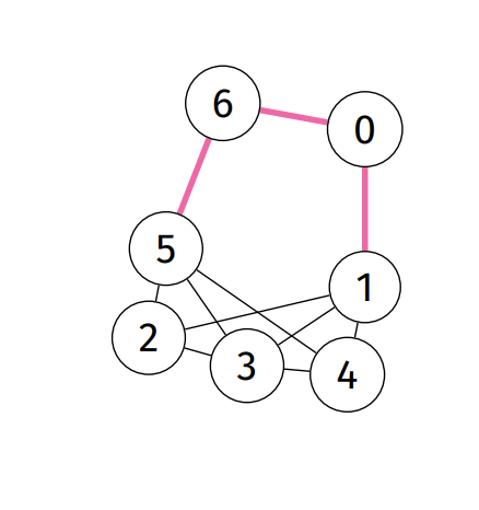
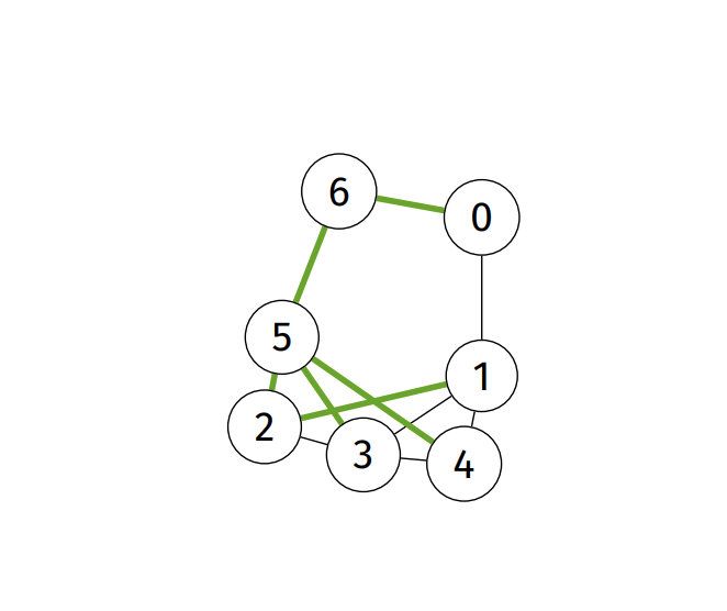
Spanning tree: (of graph) subgraph that connects all its verteces


Minimum spanning tree: spanning tree that has the least total weight


Spanning forest: (of graph) subgraph that contains all its vertices and is a set of ›trees


Clique: complete subgraph


Graph Representation


Adjacency Matrix: |V| X |V| matrix; each cell represents an edge


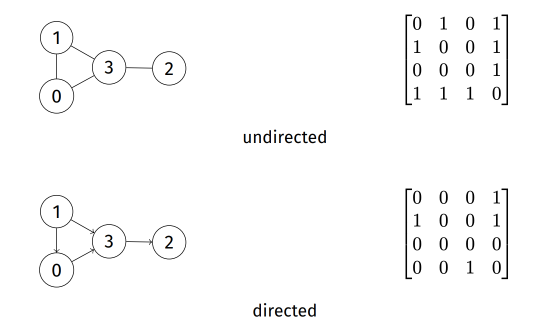
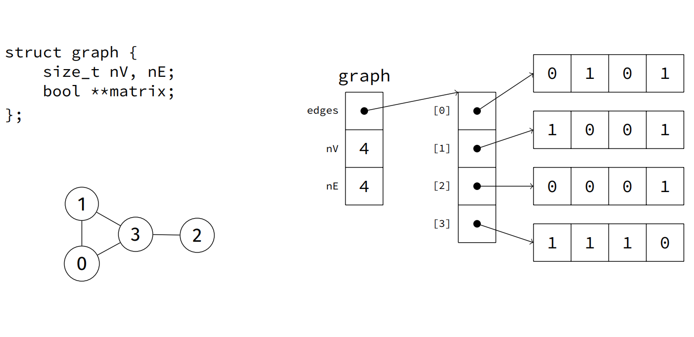
Advantages:

Easy to implement
Words for graph, digraphs, weighted fraphs, multigraphs
Time efficient


Disadvantage

Huge space: V^2
Sparce graphs ~> wasted space!
undirected graph ~> wasted space!
Inefficent initialiseation / vertex- insert/delete


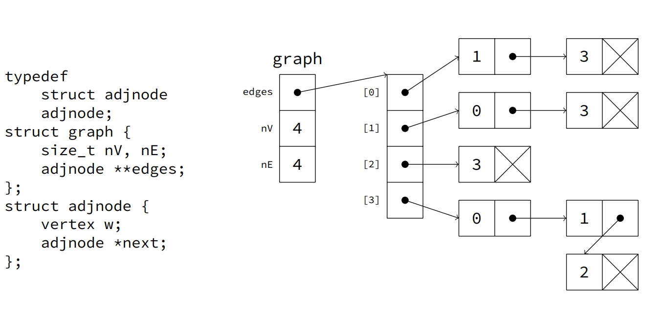
Adjacency List


Operation
Matrix
List


Space
V^2
V + E


Initialise
O(V^2)
O(V)


Destroy
O(V)
O(E)


Insert Edge
O(1)
O(V)


Find / Remove Edge
O(1)
O(V)


Is Isolated
O(V)
O(1)


Degree
O(V)
O(E)


Is Adjaceny
O(1)
O(V)


Graph ADT

typedef struct graph *Graph;

/** A concrete edge type. */
typedef struct edge { vertex v, w; weight n; } edge;

/** Create a new instance of a Graph. */
Graph graph_new (
    size_t max_edges, /**< maximum value hint */
    size_t max_vertices, /**< maximum value hint */
    bool directed, /**< true if a digraph */
    bool weighted /**< true if edges have weight */
);

/** Deallocate resources used by a Graph. */
void graph_drop (Graph g);
Graph Search (DFS / BFS)


Problem: Does a path exist between vertex v and w?


Generic Solution

Examine vertices adjacent to v;
if any of them is w, we're done
otherwise, check all the adjacent vertices and repeat util we reach w


Simple pattern:

Create a structure that will tell us what node to visit next.
Add the starting node to that structure
While that structure is not empty

Get the next vertex from that structure
Mark that node as visited (if it isn't visited)
Add Neighbours to the structure


Depth First Search (DFS): Longest paths first ~ uses a Stack

Keep track of

count: number of verticies traversed so far
pre: order in which vertices were visited
st: predecessor of each vertex (for spanning tree)


Edges traversed in all graph walks form a spanning tree, which has

edges corresponding to call-tree of recursive function
is the original graph sans cycles / alternate graph
in general, spanning tree has all vertices and a minimal set of edges to produce a connected graph (ie. no loops, cycles, parallel edges)


If a graph is not connected, DFS will produce a spanning forest
An edge connecting a vertex with an ancestor in the DFS tree that is not its parent is a back edge


Breath First Search (BFS): Adjacent nodes first ~ uses a Queue


Dikstra: Lowest-cost paths first


Directed Graphs


v -> w
eg. follow on twitter / instagram
In a digraph, edges have direction, self-loops are allowed, parallel edges are allowed
in-degree: number of directed edges leading into a vertex

source: a vertex with a in-degree 0;


out-degree: number of directed edges leading out of a vertex

sink: a vertex with out-degree 0;


reachability: indicates existence of directed graph

if a direct path v,...w exists
w is reachable from v.


strongly connected:

if both paths v,...,w and w,...,v exist then v and w are strongly connected


strongly connected: indicates mutual reachability

if both paths v,...,w and w,...,v exist
v and w are strongly connected


strong connectivity: every vertex reachable from every other vertex
strongly-connected component: maximal strongly-connected subgraph
Representations

Adjacency matrix ... Asymmetrix, sparese, less space efficent
Adjaceny List... Fairly common
Edge lists... Order of edge components matters
Linked data structures.. pointers inherently directional


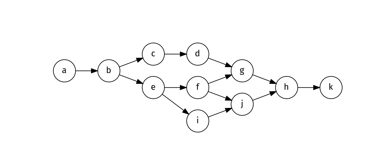
DAGs: Directed Acyclic Graph

Tree like where each vertex has children
Graph like where child vertex may have multiple parents


Weighted Graphs


Sometimes we need to assign a cost to a relationship between nodes (ie. distances between two map locations)
We use geometric interpretation

low weight -> short edge
high weight -> high edge


Sometimes weights can be negative
Representations

Adj Matrix: store weight in each cell (not just bool)

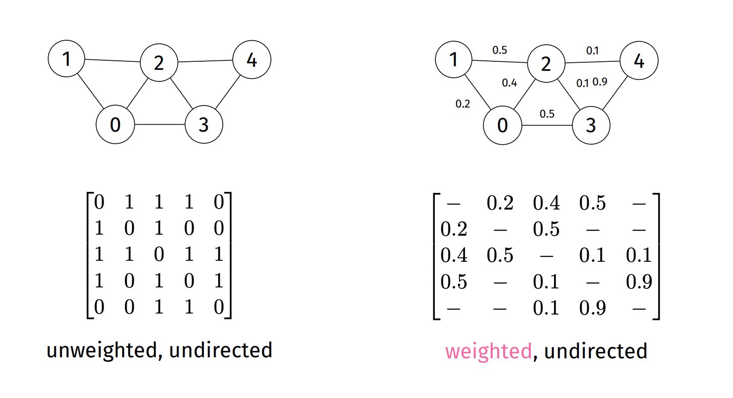
Adj List: Add weight attribute to each list node
Edge List: Add weight to each edge
Linked data structure: links become link/weight pairs


Shortest path problem:

Find the minimum cost path between two vertices
Edges may be directed or undirected
Assuming non-negative weights


Minimum Spanning Trees

Find the weight-minimal set of edges that connects all vertices
Multiple solutions may exist
Assuming undirected, non-negative weighted graphs


Shortest Path Search

source-target: shortest path from v to w
single-source: the shortest path from v to all other verices
all-pairs: the shortest paths for all pairs of v, w
Note: If no weights we use least hops


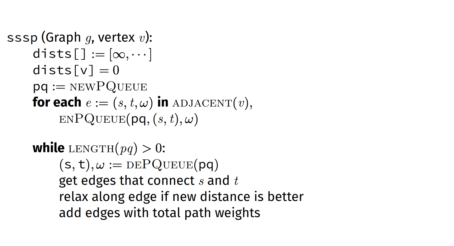
Edge relaxation along edge e from s to t:

dist[s] is length of some path from v to s
dist[t] is length of some path from v to t
if e gives shorter path v to t via s, update dist[t] and st[t].
basically update the distance and spanning tree if a shorter path has been found.


Complexity:

Using Adj List: O(E log V)
Using Adj Matrix: O(V^2)
Same as BFS/DFS but using a PQueue


MSTs


Applications:

Routing and network layout
Economical construction of electric power network


Kruskal: grow many forests

Algo

Take all edges and sort according to weight
For each edge add to new graph, unless it introduces a cycle


Cycle checking is really expensive
Sorting: O(E log E)
Prim: Maintain a connectivity frontier

Algo

Start from any vertex s with an empty MST
Choose edge not already in MST to add

Must not contain a self-loop
Must connect to a vertex already on MST
Must have minimal weight of all such edges


Check to see whether adding the new edge brought any of the non-tree vertices closer to the MST
Repeat until MST has all vertices


Easy Algo

Start with any edge
Choose edge with least weight

Add to MST


Check what edges connect to all visited nodes, with least weight (without visiting previously visited node)

Add to MST
GOTO (3. ~ ie. repeat until all vertices have been visited)


O (E log V)
Basically dijkstra's SSSP algorithm


Computability


Hamilton Paths and Tours

Hamilton path: path in graph that visits each vertex exactly once.
Hamilton tour: hamiltonian path that's a cycle.
BRUTE FORCE! enumerate every possible path, and check each one

Hack a BFS or DFS to do it
Keep a counter of vertices visited in current path
Only accept a path if count is equal to the number of verticies
Must inspect every possible path in graph = (V/e)^V
NP problem (non-deterministic polynomial)


Euler Paths and Tours

Euler path: path in graph that visits every edge exactly once. Starts and ends with different vertices.

Exactly two verticies of odd degree


Euler tour: path in graph that uses every edge of a exactly once. Starts and ends on same vertex.

All verties of even degree


Can be found in linear time


Tractable Problems

Can we find a simple path connecting two vertices in a graph?
What's the shortest path?
Given two colors, can we colour every vertex in a graph such that no two adjacent vertices are the same colour?
Is there a clique in a given graph?


Intractable Problems

What's the longest path
Given three colors, can we colour every vertex in a graph such that no two adjacent vertices are the same colour?
What's the largest clique


Graph Isomorphism: Can we make two given graphs identical by renaming verticies?

No general solution exists...


Sorting


Analysing sorting algorithms:

N: number of items (hi + lo + 1)
C: number of comparisons between items
S: the number of times items are swappped


Aim to minimise C and S
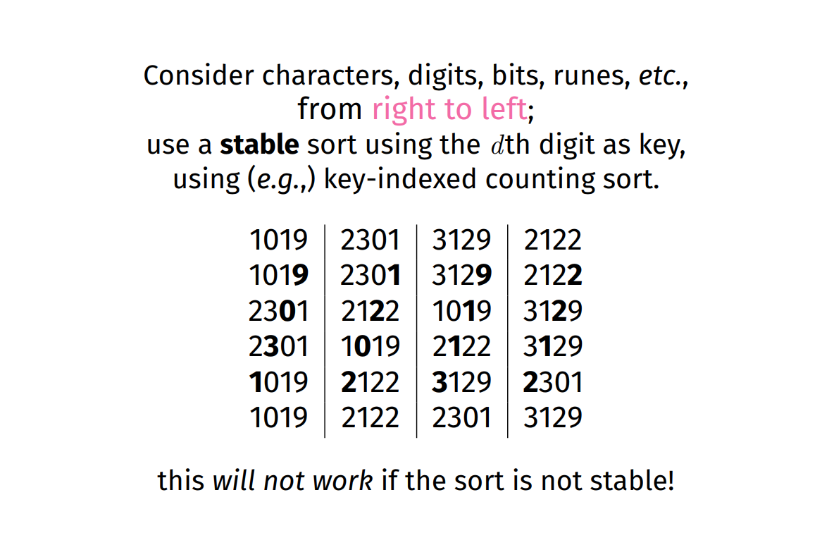
Stable: Doesn't change relative order of elements with same key
Inplace: Modifies original array

Bubble Sort (Stable)


Steps:

Swap adjacent nodes if left > right
Repeat the above


best: O(n^2)
worst: O(n^2)
stable / in place
Adaptive (Optional - early exit if sorted) ~ best: O(n)

Selection Sort


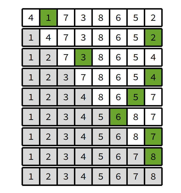
Steps:

Select the smallest element.
Swap it with first position.
Repeat above with first position increased and search boundry decreased.


best: O(n^2)
worst: O(n^2)


Insertion Sort (Stable)


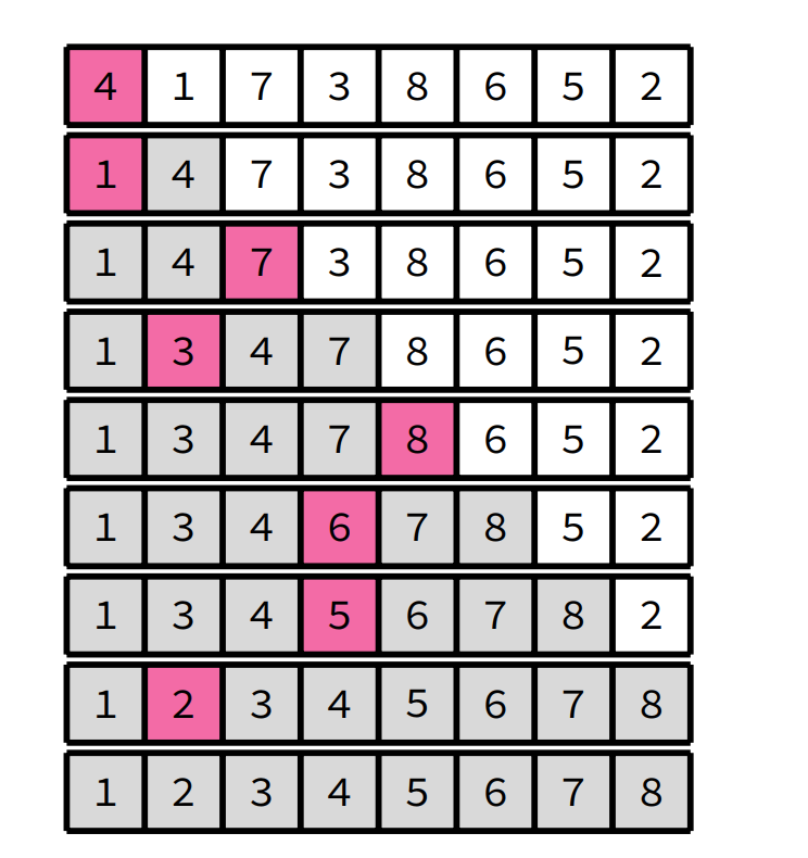
Steps:

Take the first element, insert into the first position.
This is the start of our sorted sublist
Take the next element, insert into the sorted sublist, in the right spot!
Repeat until sorted!


Shell Sort


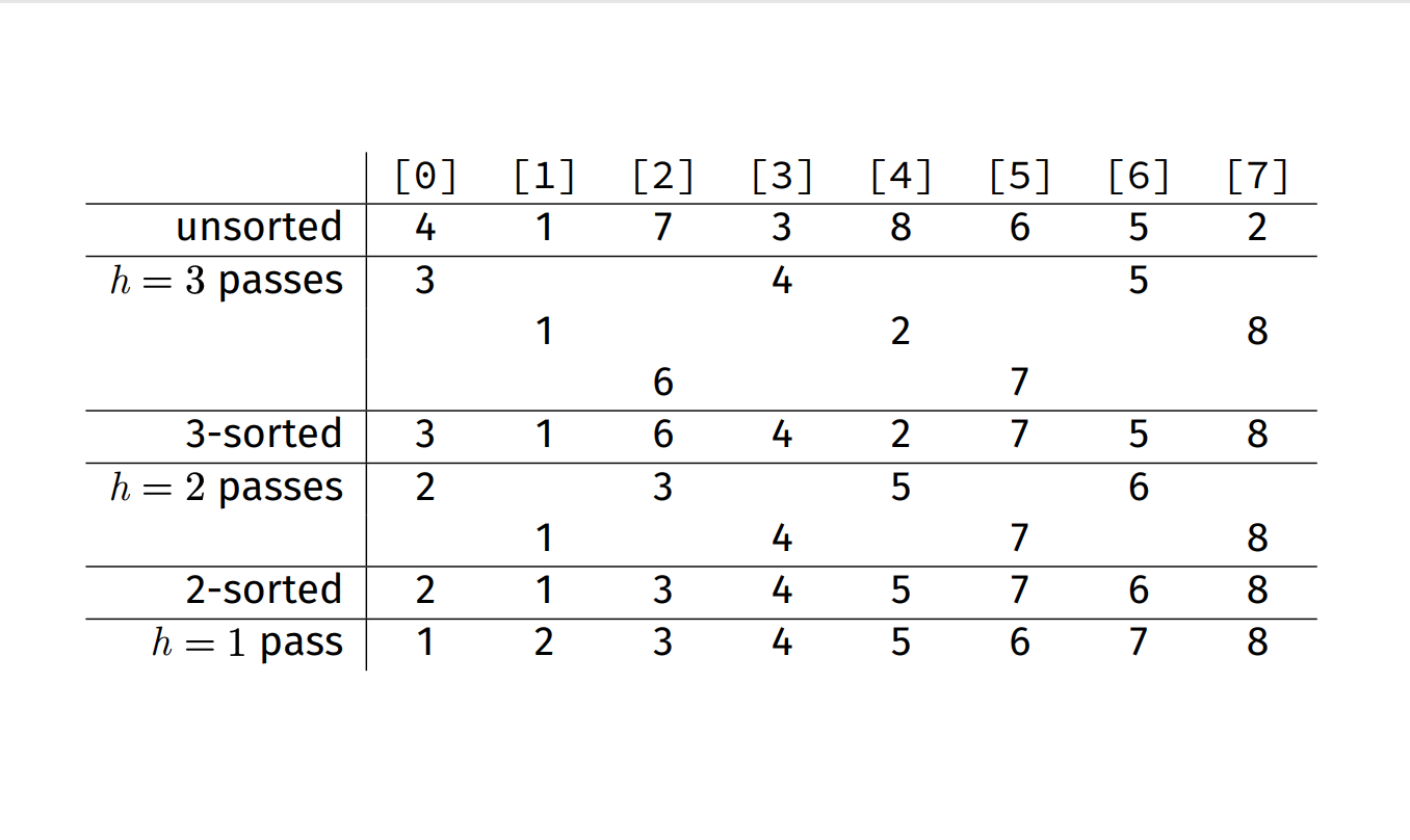
Steps:

Initialize the value of h (hilbert series)

h = 1, h <= (n-1) / 9, h = (h*3) + 1
ie. 1, 4, 13, 40...


Divide the list into smaller sub-list of equal interval h
Sort these sub-lists using insertion sort
Repeat until complete list is sorted
h=1 is an insertion sort


https://www.youtube.com/watch?v=j818Yud-ruc


Merge Sort


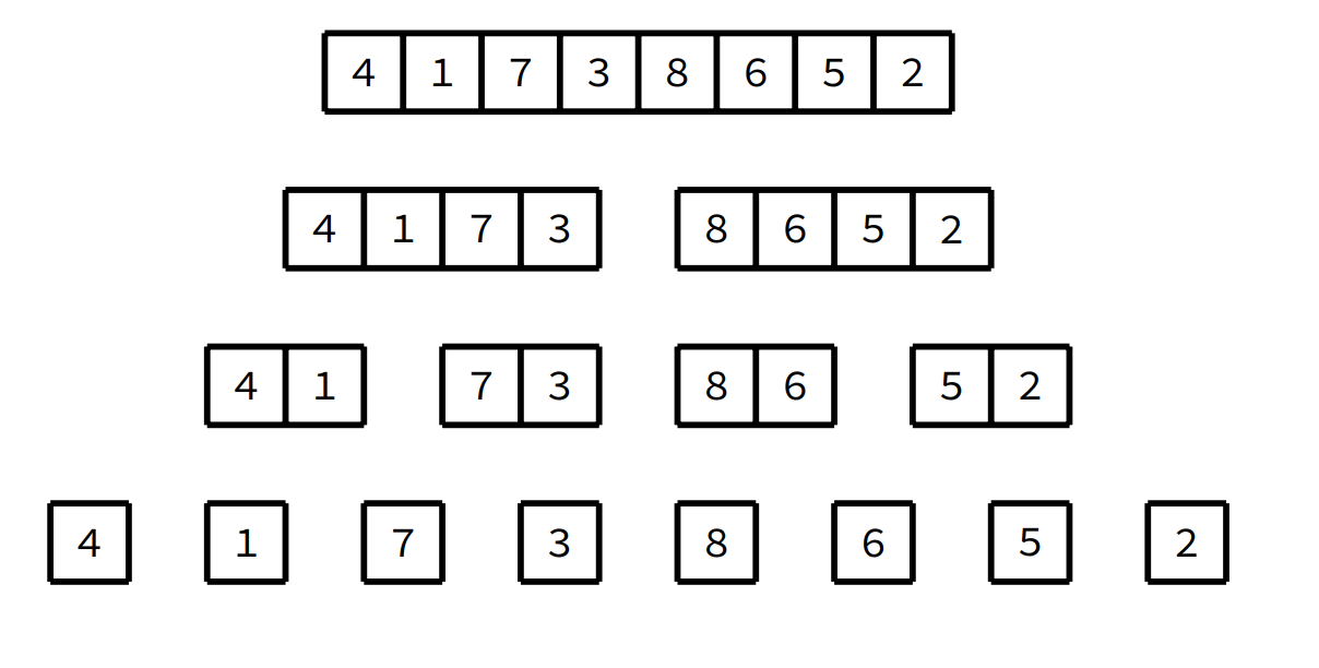
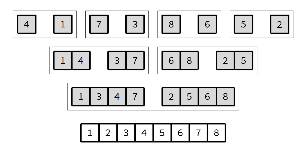
Divide and conquer


Steps:

Partion the input into two equal size parts.
Recursively sort each of the partitions.
Merge the two sorted partitons back together.


https://www.youtube.com/watch?v=JSceec-wEyw


Worst: O(n log n)


Merge sort uses a trivial split operation


Most of the work is done in the merge operation

ie. end = MIN(i + 2*m - 1, hi)


Quick Sort


Divide and conquer
Pivot

Correct position in final, sorted array
Items to left are smaller
Items to right are larger


Partition / Pivot Steps

Choose the highest index value has pivot
Take two variables to point left and right of the list excluding pivot
left points to the low index
right points to the high
while value at left is less than pivot move right
while value at right is greater than pivot move left
if both step 5 and step 6 does not match swap left and right
if left ≥ right, the point where they met is new pivot


Quick sort steps

Make the right-most index value pivot
partition the array using pivot value
quicksort left partition recursively
quicksort right partition recursively


Unstable
Choosing a pivot:

Something that divides the array in half (or as close as possible)
M-O-3: use the middle value of array a[lo, mid, hi] as the pivot, where a[lo] <= a[mid] <= a[hi]


O(log n) best case
M-O-3 / random: O(n log n) worst & avg case

Key-Indexed (Counting sort)


Non-comparison
Just access keys based on ordered values
O(n) worst case

Heap


Non-comparison
Steps:

Add all items to pqueue (implemented as heap).
Remove items from pqueue into original array.


best: Ω(n log(n))
worst: O(n log(n))
not stable

Radix Sort


Non-comparison
Only if we can decompose keys
Sorting individually on each part of the key at a time:

digit by digit


Time complexity O(kn)

Balanced Trees


Degenerate trees: height is at most n - 1   <- We're trying to avoid this

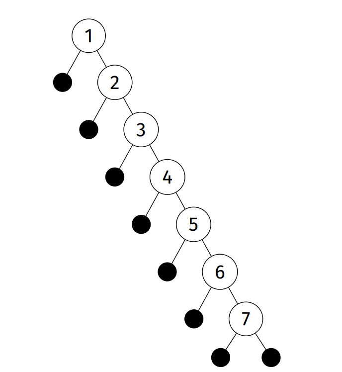
Ascending-ordered or descending ordered is a pathalogical case


Balanced trees: height is at least log n

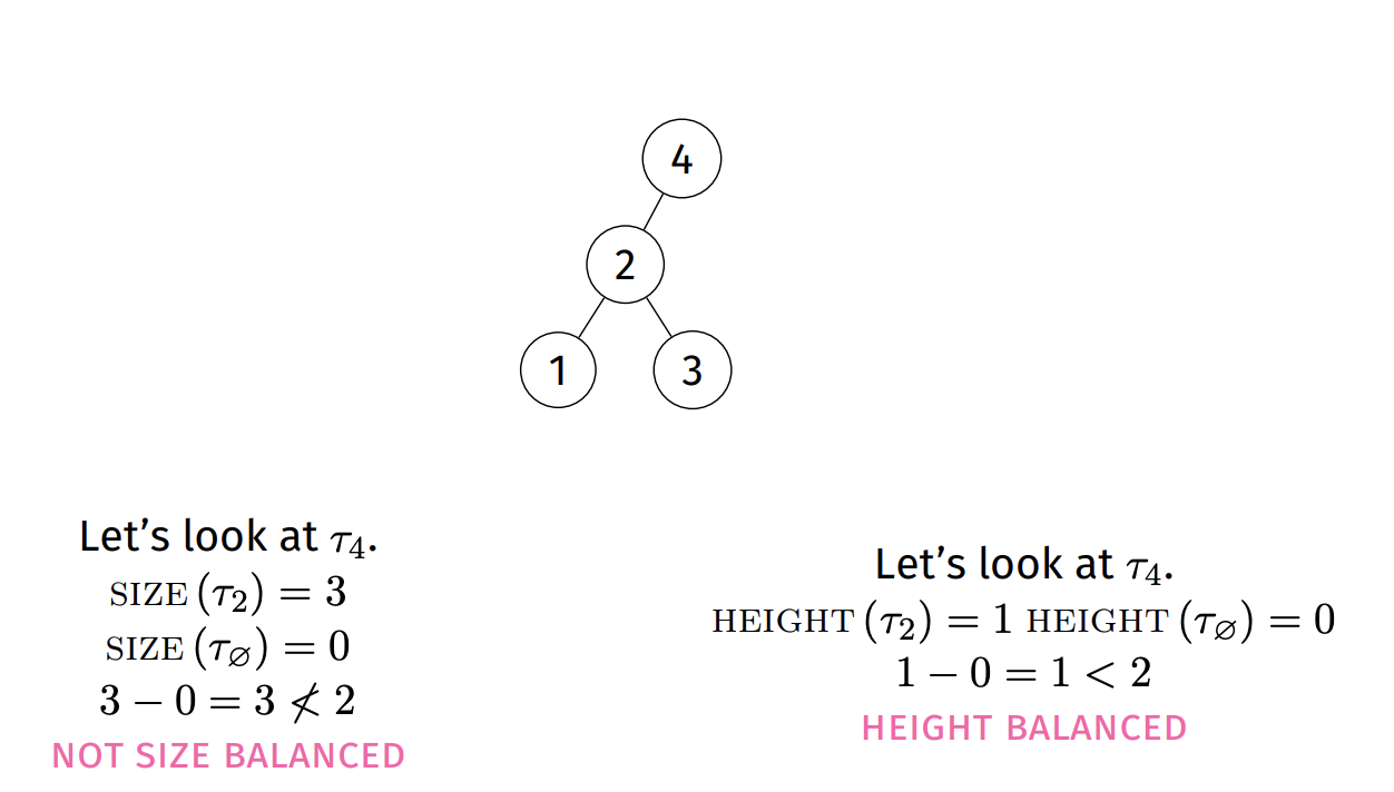
Size balanced: |size(t.L) - size(t.R)| < 2
Height balanced: |height(t.L) - height(t.R)| < 2


Costs for Degenerate

Insertion ~ O(n)
Search / Deletion ~ O(n)


Costs for Balanced

Insertion ~ O(log n)
Search / Deletion ~ O(log n)


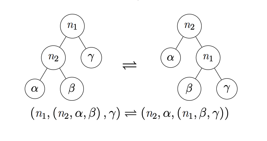
Right and Left Rotations: primitive operations that change the balance of a tree whilst maintaining a search tree


Partition is a way to brute force some balance into a tree, by lifting some kth index to the root.


Global rebalancing: move the median node to the root by partitioning on size / 2 index; then left sub tree and right subtree


btree_node *btree_balance_global (btree_node *tree)
{
    if (tree == NULL) return NULL;
    if (size (tree) < 2) return tree;
    tree = partition (tree, size (tree) / 2);
    tree->left = btree_balance_global (tree->left);
    tree->right = btree_balance_global (tree->right);
    return tree;
}


Cost for global rebalancing

Dengerate ~ O(n log n)
Balanced ~ O(n)


Local rebalancing: do small, incremental operations to improve the overall balance of the tree at the cost of imperfect balance


Amortisation: do small amount of work now to avoid more work later. (ie. splay tree operations)


Randomisation: use randomness to reduce impact of BST worst cases.


Optimisation: maintain structural information for performance. (ie. include size attribute on each node on btree)


Root insertion

How to insert a node at the root without having to rearrage all node?
Do a leaf insertion and rotate the new node up the tree
Same complexity as leaf insertion


Random insertion

We randomly choose which level to insert a node
Do a normal leaf insetion, most of the time. Random with certain probability
Do a root insertion of a value.
Basically randomly choosing to do a root insertion or note


Splay Trees


Root insertions can still leave us with a degenerate tree.
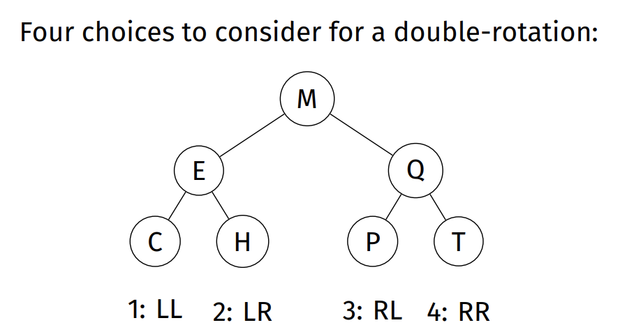
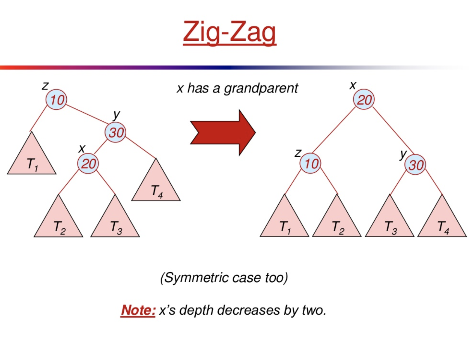
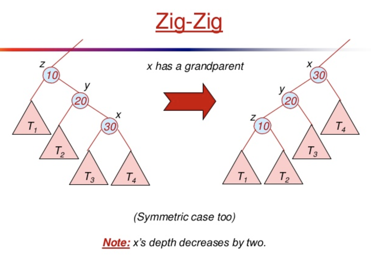
Splay trees vary root-insertion by considering three levels of the tree

parent, child, grandchild
performs double-rotations based on p-c-g orientation


Fast ACCESS TO ELEMENTS RECENTLY ACCESSED
Don't care about balance, just want the root to be most recently accessed node.
All operations: O(log n) on average / O(n) on worst case ~ n is number of nodes on tree
Any sequence of k operations, starting from empty tree, never >n tree,  any tree operation takes O(k log n), worst case time
Basis: Splay trees kepted in balance with rotations (rotate left, rotate right).
Splay trees are NOT kept perfectly balanced -> that why operations maybe O(n)

Ie. Inserting 1...n, and having to splay to root, creates a degenerate tree


Splay tree operations


3 Cases for rotating:

(Zig-Zag) X is a left child of a right child OR X is a right child of a left child.

(Zig-Zig) X is a left child of a left child OR X is a right child of a right child.

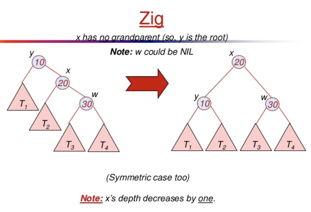
(Zig) X is a child of the root


Search (key)

Regularly to a binary search tree


Walk down a tree, deciding to walk left / right, until we reach k or a dead-end
Let X be the node where search ended, whether it contains key or not.


Splay X up the tree through a sequence of rotations, so X becomes the root


Super fast performance when searching for same key over and over again


Find Min / Max

Keep walking to the left / right
Splay last node to the root


Insert a new key and value

Insert into tree like a normal binary tree
Splay new node to the root


Remove (key)

Remove a key like a normal BST.
Keep track of actual node that got remove (ie. the left most value from right sub tree), we'll call it X
Spay X's parent to the root


2-3-4 Trees


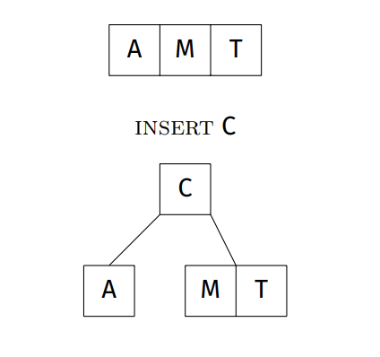
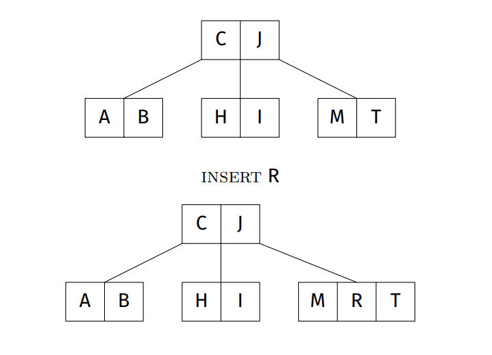
Each node can have 3 kinds of nodes:

2-nodes: 1 values ~ 2 children
3-nodes: 2 values ~ 3 children
4-nodes: 3 values ~ 4 children


Each node stores three vvalues at most (from smallest to greatest)


2-3-4 trees grow 'upwards' from the leaves all of which are equidistant to the root.


Self balancing data structure, commonly used to implement dictionaries.


Always balanced; depth is O(log n)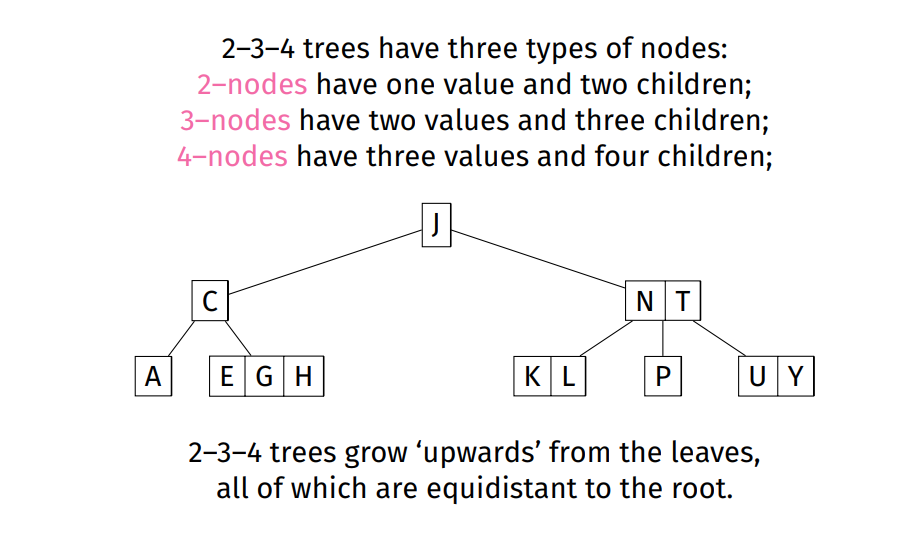


Worst case for depth: all nodes are 2-nodes ~ depth = log_2 n


Best case for depth: all nodes are 4-nodes ~ depth = log_4 n


Insertion steps

Find leaf node where item belongs (via search)
if node is not full (ie. order < 4), insert item in this node, order++
if node is full (ie. contains 3 items - 4 node)

split into two 2-nodes as leaves
promote middle element to parent
insert item into appropriate leaf 2-node
if parent is a 4-node, continue split / promote upwards
if promote to root, and root is a 4-node, split root node and add new root


Insertion examples:


Red black trees


Representations of 2-3-4 trees
Using BST nodes
Gets benefits of 2-3-4 tree self-balancing on insert, delete ...
Uses labels to tell us when to rebalance
Rules

Root Property: Root node is always black
External Propery: Every external node is always black
Red Property: Children of red nodes are black
Depth Property: All nodes have the same black depth


Fix cases

When uncle is black -> we rotate
When uncle is red -> we colour flip


Red Links:

combine nodes to represent 3 and 4 nodes
child along red link is a 2-3-4 neighbour


Black Links:

Ordinary child links


Operations

Search: O(log n)

No different from regular BST


Insert: O(log n)
Remove: O(log n)


Hash Tables


Linked list, Tree, etc... have pretty slow insert and search operations


They don't take advantage of cache locality


Hashing lets us approximate

Arbitrary keys (ie. strings etc)
Map key into a compact range of index values
Store items in array, accessed by index value
O(1)


What we need

Array of items
Hash function: hash(key) -> index
Collision resolution method (ie. when value already exists for given key)


Properties we want for the hashing function, h:

For a table size N, output range is 0 to N-1
pure, deterministic h(k,N) ~ ie. gives same result
spreads key values uniformly over index range
cheap (enough) to compute


Other properties we need for h:

Pre-image resistant: h=HASH(M), given h, hard to pick m
Second pre-image resistant: for HASH(m1) = HASH(m2), given m1, it's hard to find m2
Collision resistant: hard to find m1 and m2


What if two keys hash to the same index?

Allow for multiple items in a single location?
Systematically compute new indices by various probing strategies
Resize the array by adjusting hashing function, and rehash all values into new array


Given N slots and M items:

best case: all lists have length M/N
worst case:  one list with length M, all other 0


With good hash and M <= N, cost O(1)


With good hash and M > N, cost O(M/N)


M/N ratio is called load


Collision Resolution

Chaining

Using a linked list
Using a tree (a bit more efficent O(log n) search)


Linear Probing

If table is not close to being full, there are still many empty slots, we could just use the next available slot along

to reach first item: O(1)
to reach subsequent items, depends on load
worst case: O(N)


Double Hash Probing

If key already exists, hash again and add the new value to the incremented index (ie. index = hash1(key) + hash2(key))
Hash1 to Hash2 should be relatively prime to each other, and to N
Faster than linear probing
MUST NEVER BE EVALUATED TO 0!!!
Choose a hash function:

P = prime number less than NSLOTS
steps = H_2(x) = P - (x % p)
Move step + h(x) ~ ie. increment steps using H_2 from original hash output


Resize table

You'll need to rehash and insert into table again.


Performance:

Good HASH function is critical
Choosing a good N for M is critical (ie. managing the load)
Choosing a good resolution approach is critical

Linear probing is fastest, given big N!
Double hasing: faster for higher load, more efficient
Chaining: pssible for loads that are greater than 1, but degenerates


Cool Algos

Merge two linked lists in sorted order

Node MergeLists(Node list1, Node list2) {
  if (list1 == null) return list2;
  if (list2 == null) return list1;

  if (list1.data < list2.data) {
    list1.next = MergeLists(list1.next, list2);
    return list1;
  } else {
    list2.next = MergeLists(list2.next, list1);
    return list2;
  }
}
Recursive Tree Functions

// Tree clone
Tree *tree_clone (Tree t)
{
  if (!t) return t;

  Tree new = malloc(sizeof(*new));
  new->item = t->item; // copy item from tree
  new->left = tree_clone(t->left);
  new->right = tree_clone(t->left);

  return new;
}

// Tree reverse
void tree_reverse (Tree t)
{
  if (!t) return;
  
  Tree tmp = t->left;
  t->left = t->right;
  t->right = tmp;

  tree_reverse (t->left);
  tree_reverse (t->right);
}

// Check if two trees are equal
bool tree_eq (Tree t1, Tree t2)
{
    if (!t1 && !t2) return true;
    if (t1 && t2) {
        return (t1->val == t2->val)
            && tree_eq (t1->left, t2->left)
            && tre_eq (t1->right, t2->right);
    }
    return false;
}
Duplicate linked list

link list_duplicate (link l)
{
	link new;
	if (l == NULL)
		return NULL;
	new = node_new(l->item);
	new->next = list_duplicate (l->next);
	return new;
}

link dlist_duplicate (dlink l, prev)
{
	dlink new;
	if (l == NULL)
		return NULL;
	new = node_new (l->item);
    new->prev = prev;
	new->next = list_duplicate (l->next, l);
	return new;
}
Operation	Matrix	List
Space	V^2	V + E
Initialise	O(V^2)	O(V)
Destroy	O(V)	O(E)
Insert Edge	O(1)	O(V)
Find / Remove Edge	O(1)	O(V)
Is Isolated	O(V)	O(1)
Degree	O(V)	O(E)
Is Adjaceny	O(1)	O(V)