01/13/2012. From a lecture by Professor John Ousterhout at Stanford, class CS140
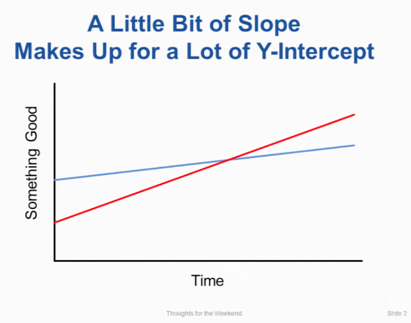
Here's today's thought for the weekend. A little bit of slope makes up for a lot of Y-intercept.
[Laughter]
| ### Title: Back to basics: High quality plots using base R graphics | |
| ### An interactive tutorial for the Davis R Users Group meeting on April 24, 2015 | |
| ### | |
| ### Date created: 20150418 | |
| ### Last updated: 20150423 | |
| ### | |
| ### Author: Michael Koontz | |
| ### Email: mikoontz@gmail.com | |
| ### Twitter: @michaeljkoontz | |
| ### |
| library(ggplot2) | |
| library(dplyr) | |
| library(tidyr) | |
| library(stringr) | |
| library(scales) | |
| library(gridExtra) | |
| library(grid) | |
| # use the NPR story data file --------------------------------------------- | |
| # and be kind to NPR's bandwidth budget |
| library(emmeans) | |
| data(mtcars) | |
| # in the example here, all models give the same point estimates and similar | |
| # SEs because there is only a single, categorical, variable in the model. | |
| # if you add a continuous predictor, they will no longer, because the relationship | |
| # assumed by the model will be different for the three models! | |
| m <- glm(am ~ vs, data = mtcars, family = binomial) | |
| em1 <- emmeans(m, "vs") |