speed-test-monet-sqlite-r.Rmd

```{r}
library(MonetDBLite)
library(RSQLite)
library(DBI)
library(dplyr)

library(microbenchmark)
library(ggplot2)
```

Load 10M international events.   This is a tidy version of the events 
downloadable from https://dataverse.harvard.edu/dataset.xhtml?persistentId=hdl:1902.1/FYXLAWZRIA ([King and Lowe, 2003](http://dx.doi.org/10.1017/S0020818303573064)).

Size as a single `.rda` file on disk: *96.5M*

```{r}
load("events-1990-2004.rda")   

# adjust column names for easier SQL import
names(events) <- c("id", "xid", "sid", "eid", "place",
                   "eventdate", "eventform", "srcname",
                   "srcsector", "srclevel", "tgtname",
                   "tgtsector", "tgtlevel")
```
Set up a Monet database in a local directory, make events a table,
and create a table front for dplyr

```{r}
dbdir <- "monet-dplyr-dir"
con1 <- dbConnect(MonetDBLite::MonetDBLite(), dbdir)
dbWriteTable(con1, "events", events, overwrite = TRUE)
ev1 <- tbl(con1, "events")
```

Size as a folder on disk: *425M* 

Set up an SQLite database in a local directory, make events a table and 
create a table front for dplyr

```{r}
dbfile <- "sqlite-dplyr.db"
con2 <- dbConnect(RSQLite::SQLite(), dbfile)
dbWriteTable(con2, "events", events, overwrite = TRUE)
ev2 <- tbl(con2, "events")
```

Size as a single sqlite file on disk: *690M*

Set up an SQLite database in memory and create a table from for dplyr

```{r}
con3 <- dbConnect(RSQLite::SQLite(), ":memory:")
dbWriteTable(con3, "events", events, overwrite = TRUE)
ev3 <- tbl(con3, "events")
```

Set up an SQLite database in memory and create a table from for dplyr

```{r}
con4 <- dbConnect(RSQLite::SQLite(), ":memory:")
copy_to(con4, events, "events",
        indexes = list("eventform"))
ev4 <- tbl(con4, "events")
```

We'll test a single variable tabulation.  Here are the test functions:

```{r}
# Base R's version, using table
timing_r <- function(ev){ 
  table(ev$eventform) 
}

# SQL via DBI version
timing_dbi <- function(con){
  rr <- dbSendQuery(con, "SELECT eventform, COUNT(eventform) FROM events GROUP BY eventform")
  res <- dbFetch(rr)
  dbClearResult(rr)
}

# dplyr version
timing_dplyr <- function(ev){
  ev %>%
  select(eventform) %>%
  group_by(eventform) %>%
  summarise(count = n()) %>%
  collect()
}
```

Run the test.  This takes about 12 minutes on my laptop

```{r}
res <- microbenchmark(r = timing_r(events),
                      dbi1 = timing_dbi(con1),
                      dbi2 = timing_dbi(con2),
                      dbi3 = timing_dbi(con3),
                      dbi4 = timing_dbi(con4),
                      dplyrr = timing_dplyr(events), 
                      dplyr1 = timing_dplyr(ev1),
                      dplyr2 = timing_dplyr(ev2),
                      dplyr3 = timing_dplyr(ev3),
                      dplyr4 = timing_dplyr(ev4),
                      times = 30)
```

and close up the connections now we're done.

```{r}
dbDisconnect(con1, shutdown = TRUE)
dbDisconnect(con2, shutdown = TRUE)
dbDisconnect(con3, shutdown = TRUE)
dbDisconnect(con4, shutdown = TRUE)
```


Results:

```{r}
tab <- summary(res) %>% 
  mutate(library = case_when(
                     grepl("dbi", expr) ~ "DBI", 
                     grepl("dplyr", expr) ~ "dplyr", 
                     expr == "r" ~ "base"), 
         database = case_when(
                      grepl("1", expr) ~ "Monet", 
                      grepl("2", expr) ~ "SQLite (disk)", 
                      grepl("3", expr) ~ "SQLite (memory)", 
                      grepl("4", expr) ~ "SQLite (memory+index)", 
                      TRUE ~ ""),
         seconds = time / 1000000000,
         Condition = paste(library, database)) 
```
Speed summaries (in milliseconds)


|        min|        lq|      mean|    median|        uq|       max| neval|library |database              |
|----------:|---------:|---------:|---------:|---------:|---------:|-----:|:-------|:---------------------|
|  654.82496|  908.8472|  990.2477|  970.7917| 1064.4448| 1526.8617|    30|base    |                      |
|   98.51502|  127.3214|  143.2917|  138.8620|  157.6495|  218.0188|    30|DBI     |Monet                 |
| 5227.39406| 5273.4724| 5315.1499| 5306.2525| 5338.7910| 5485.8420|    30|DBI     |SQLite (disk)         |
| 5084.73081| 5101.5085| 5136.9485| 5123.0648| 5140.5585| 5326.1279|    30|DBI     |SQLite (memory)       |
|  882.60921|  890.9514|  907.7341|  897.7100|  909.2202| 1003.5088|    30|DBI     |SQLite (memory+index) |
|  413.31117|  429.5574|  473.0778|  436.2304|  445.9132| 1433.8018|    30|dplyr   |                      |
|  113.06272|  150.7392|  165.2783|  164.3106|  187.6424|  237.1465|    30|dplyr   |Monet                 |
| 5127.23870| 5156.3244| 5186.5221| 5178.9403| 5206.6186| 5369.7247|    30|dplyr   |SQLite (disk)         |
| 4949.46828| 4988.3494| 5016.4259| 5010.3839| 5034.5425| 5235.0919|    30|dplyr   |SQLite (memory)       |
|  762.09109|  768.8625|  778.1123|  774.8939|  782.2196|  823.0093|    30|dplyr   |SQLite (memory+index) |

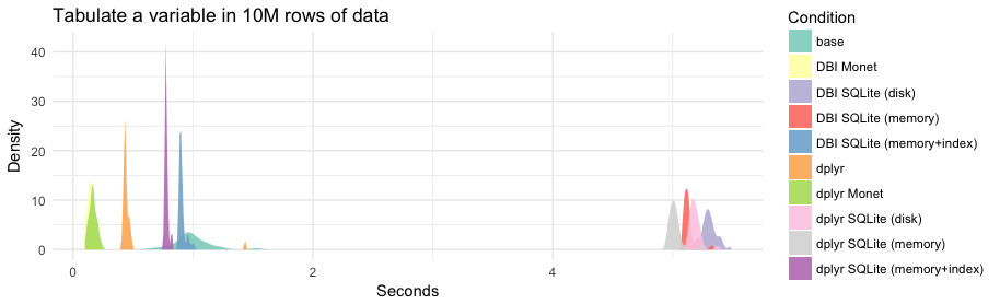
```{r}
theme_set(theme_minimal())
ggplot(tablong, aes(x = seconds, fill = Condition)) + 
  geom_density(alpha = 0.9, col = NA) + 
  scale_fill_brewer(palette = "Set3") + 
  labs(title = "Tabulate a variable in 10M rows of data",
       x = "Seconds", y = "Density")
```

![speed-test](https://user-images.githubusercontent.com/509288/43366563-d3f9a39a-930d-11e8-963e-6f089a69ee31.png)

OK some extras. What about data.table?

Well, I don't really know what I'm doing with data.table but it seems like the test function should be something like

# convert to a data.table
dt_events <- as.data.table(events)

# do the group by and count
timing_dt <- function(dt){
  dt[, .N, by=eventform]
}

and if that's reasonable usage then the R, dplyr, and data.table timings come out like

res0 <- microbenchmark(r = timing_r(events),
                      dplyrr = timing_dplyr(events),
                      dt = timing_dt(dt_events),
                      times = 30)

expr	min	lq	mean	median	uq	max	neval
r	557.5196	744.3698	893.1391	902.8652	977.9563	1868.7553	30
dplyrr	425.5445	434.6060	469.1267	446.6652	458.8747	798.9253	30
dt	126.2017	153.0440	196.1584	156.9442	162.6290	517.7313	30

So data.table is competitive (maybe a tad slower than) Monet, when accessed by DBI.