This paper:
Finding the number of clusters in a data set: An information theoretic approach
CATHERINE A. SUGAR AND GARETH M. JAMES
Marshall School of Business, University of Southern California
...is fascinating. Let's work through its ideas by implementing its methods and replicating its examples.
You should read the paper, or at the very least the abstract, but for those that refuse to do so, the gist I'll repeat here is that we can use ideas from information theory to evaluate choices for the number of clusters (which we refer to as k) in data sets we apply the k-means clustering algorithm to.
Don't try to read the paper alongside this document: the narrative here does not match the order in which Sugar & James introduce concepts and data sets. I don't intend for this to be read alongside the paper, but rather as a different path for exploring the ideas they introduce, so I recommend reading or skimming the paper first before working through this document.
So, what does it mean to apply information theory, specifically rate distortion theory, to clustering applications? The core idea is actually quite concise. The authors describe it in section 2.1:
One can characterize cluster analysis as an attempt to find the best possible representation of a population [that is, of a data set —DL] using a fixed number of points. This can be thought of as performing data compression or quantization on i.i.d. [independently and identically distributed] draws from a given distribution.
Awesome! Clustering a set of data is like summarizing it. And this tells us directly what it means (like, philosophically) to select the number of clusters: we're looking for that ideal balance between compressing the original information and retaining its meaning. For more on this general concept (as Sugar & James note), see the work of Claude Shannon (including this short Clojure-based walkthrough).
By modeling clustering as a kind of compression, Sugar & James provide a tool to better determine which choice of k is best suited to a given data set. That is, they propose a method to determine how many clusters best describe a data set.
With that conceptual understanding in hand, let's look at some concrete applications. If you like, you can open the Clojure version of this file, fire up a REPL, and evaluate as you read.
Let us begin with that old classic, Fisher's iris data. We direct Incanter to grab it for us. (The next few lines about PCA are directly from Data Sorcery with Clojure, modified only to :require Incanter rather than use.)
;; The namespace we're going to use will need these:
(:require [incanter.core :as i]
          [incanter.stats :as incs]
          [incanter.charts :as incc]
          [incanter.datasets :as incd]
          [clj-ml.clusterers :as mlc]
          [clj-ml.data :as mld])

(def iris (i/to-matrix (incd/get-dataset :iris)))
Since the iris data is multivariate, to plot it as an xy graph we must condense its attributes. For that we perform principal component analysis (PCA):
(def X (i/sel iris :cols (range 4)))
(def components (:rotation (incs/principal-components X)))
(def pc1 (i/sel components :cols 0))
(def pc2 (i/sel components :cols 1))
And now we can view the four-dimensional iris data in two dimensions. We group by species using color.
(i/view (incc/scatter-plot (i/mmult X pc1) (i/mmult X pc2)
                           :group-by (i/sel iris :cols 4)
                           :x-label "PC1"
                           :y-label "PC2"
                           :title "Iris PCA grouped by species [Figure 5c]"))
...which should look like this:
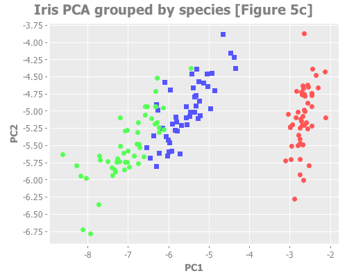
So, we know that this data forms three groups by species, but visualizing it with PCA reveals that while one species is well differentiated, the other two have overlapping attributes. Therefore this data could legitimately be interpreted as consisting of either two or three groups.
Let's now explore what k-means analysis and Sugar & James' approach say about the iris data. We'll use WEKA's k-means implementation via its Clojure wrapper, clj-ml. I've already aliased its 'clusterers' and 'data' namespaces as mlc and mld respectively, so we can get started.
(def iris-kmeans-2 (mlc/make-clusterer :k-means {:number-clusters 2}))What we have here is a 'clusterer' object, which one uses in WEKA to perform cluster analysis. (It's a rather object-oriented approach.) This clusterer doesn't say much, because while it's been created, it hasn't yet been built:
iris-kmeans-2

 => #object[weka.clusterers.SimpleKMeans 0x3b416f01 "No clusterer built yet!"]
So let's build it!
(doto iris-kmeans-2
  (mlc/clusterer-build (mld/make-dataset "Fisher's Irises"
                                         [:sepal-length :sepal-width
                                          :petal-length :petal-width]
                                        ; Withold the species column
                                        ; because not to would be
                                        ; cheating:
                                         (i/to-vect (i/sel iris :cols (range 4))))))

=> #object[weka.clusterers.SimpleKMeans 0x3b416f01 "\nkMeans\n======\n\nNumber of iterations: 5\nWithin cluster sum of squared errors: 18.37779075053819\n\nInitial staring points (random):\n\nCluster 0: 6.1,2.9,4.7,1.4,1\nCluster 1: 6.2,2.9,4.3,1.3,1\n\nMissing values globally replaced with mean/mode\n\nFinal cluster centroids:\n                            Cluster#\nAttribute       Full Data          0          1\n                    (150)      (100)       (50)\n===============================================\nsepal-length       5.8433      6.262      5.006\nsepal-width        3.0573      2.872      3.428\npetal-length        3.758      4.906      1.462\npetal-width        1.1993      1.676      0.246\nspecies                 1        1.5          0\n\n\n"]
Yow, that's hard to read. (println iris-kmeans-2) evaluates to nil but pretty-prints in the REPL:
#object[weka.clusterers.SimpleKMeans 0x1b5c3bc
kMeans
======
Number of iterations: 7
Within cluster sum of squared errors: 12.127790750538196
Initial staring points (random):
Cluster 0: 6.1,2.9,4.7,1.4
Cluster 1: 6.2,2.9,4.3,1.3
Missing values globally replaced with mean/mode
Final cluster centroids:
                            Cluster#
Attribute       Full Data          0          1
                    (150)      (100)       (50)
===============================================
sepal-length       5.8433      6.262      5.006
sepal-width        3.0573      2.872      3.428
petal-length        3.758      4.906      1.462
petal-width        1.1993      1.676      0.246 ]
So WEKA's k-means function dutifully fulfilled its task and gave us two clusters. As the Turks say, çok iyi! Let's try with 3:
(def iris-kmeans-3 (mlc/make-clusterer :k-means {:number-clusters 3}))

(doto iris-kmeans-3
  (mlc/clusterer-build (mld/make-dataset "Fisher's Irises"
                                         [:sepal-length :sepal-width
                                          :petal-length :petal-width]
                                         (i/to-vect (i/sel iris :cols (range 4))))))

(println iris-kmeans-3)

=> #object[weka.clusterers.SimpleKMeans 0x6a3536e9
   kMeans
   ======
   Number of iterations: 6
   Within cluster sum of squared errors: 6.982216473785234
   Initial staring points (random):
   Cluster 0: 6.1,2.9,4.7,1.4
   Cluster 1: 6.2,2.9,4.3,1.3
   Cluster 2: 6.9,3.1,5.1,2.3
   Missing values globally replaced with mean/mode
   Final cluster centroids:
                               Cluster#
   Attribute       Full Data          0          1          2
                       (150)       (61)       (50)       (39)
   ==========================================================
   sepal-length       5.8433     5.8885      5.006     6.8462
   sepal-width        3.0573     2.7377      3.428     3.0821
   petal-length        3.758     4.3967      1.462     5.7026
   petal-width        1.1993      1.418      0.246     2.0795 ]
Again, WEKA dutifully gives us three clusters. But how do we know which choice of k is more accurate? More true? More illuminating? We could visually compare the cluster results to each other and to the species results we already know. So, let's look at the cluster assignments WEKA made.
(.getAssignments iris-kmeans-2)Ach nein! We got an unhandled java.lang.Exception. From the stacktrace:
"The assignments are only available when order of instances is preserved (-O)"
OK, so we have to re-run our k-means analysis, this time setting a new parameter:
(def iris-kmeans-2 (mlc/make-clusterer :k-means {:number-clusters 2
                                                 NEW PARAMETER:
                                                 :preserve-instances-order true}))

(def iris-kmeans-3 (mlc/make-clusterer :k-means {:number-clusters 3
                                                 NEW PARAMETER:
                                                 :preserve-instances-order true}))
Now, before we used clj-ml's (clusterer-build), which simply wraps .buildClusterer, but since we're already Java-aware with (doto) and it doesn't add any functionality I don't see any advantage of doing so. To me, calling .buildClusterer directly is more clear:
(doto iris-kmeans-2
  (.buildClusterer (mld/make-dataset "Fisher's Irises"
                                     [:sepal-length :sepal-width
                                      :petal-length :petal-width]
                                     (i/to-vect (i/sel iris :cols (range 4))))))

(doto iris-kmeans-3
  (.buildClusterer (mld/make-dataset "Fisher's Irises"
                                     [:sepal-length :sepal-width
                                      :petal-length :petal-width]
                                     (i/to-vect (i/sel iris :cols (range 4))))))
And now?
(.getAssignments iris-kmeans-2)
=> #object["[I" 0x2b78a89b "[I@2b78a89b"]
Ah. Bien sur. So much better. o_O
It turns out we need to iterate over those assignments. And manually fold them back into our data. Oh, Java.
(def iris-2-clusters (map conj (i/to-vect iris) (.getAssignments iris-kmeans-2)))
Let's take a quick look to see if we're going in the right direction:
(take 10 iris-2-clusters)

=> ([5.1 3.5 1.4 0.2 0.0 1]
    [4.9 3.0 1.4 0.2 0.0 1]
    [4.7 3.2 1.3 0.2 0.0 1]
    [4.6 3.1 1.5 0.2 0.0 1]
    [5.0 3.6 1.4 0.2 0.0 1]
    [5.4 3.9 1.7 0.4 0.0 1]
    [4.6 3.4 1.4 0.3 0.0 1]
    [5.0 3.4 1.5 0.2 0.0 1]
    [4.4 2.9 1.4 0.2 0.0 1]
    [4.9 3.1 1.5 0.1 0.0 1])
Cool.
(def iris-3-clusters (map conj (i/to-vect iris) (.getAssignments iris-kmeans-3)))OK. We're all set to compare k=2 and k=3 for the iris data. We reach for PCA again, re-using our existing definitions of X, pc1, and pc2, but grouping now not by species but by cluster assignment.
(i/view (incc/scatter-plot (i/mmult X pc1) (i/mmult X pc2)
                           :group-by (i/sel (i/to-matrix (i/to-dataset iris-2-clusters))
                                            :cols 5)
                           :x-label "PC1"
                           :y-label "PC2"
                           :title "Iris PCA grouped by 2 k-means clusters"))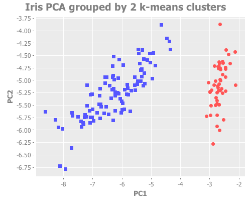
(i/view (incc/scatter-plot (i/mmult X pc1) (i/mmult X pc2)
                           :group-by (i/sel (i/to-matrix (i/to-dataset iris-3-clusters))
                                            :cols 5)
                           :x-label "PC1"
                           :y-label "PC2"
                           :title "Iris PCA grouped by 3 k-means clusters"))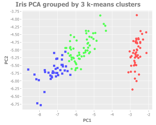
From a purely visual standpoint, I'd say both of these are excellent clustering attempts. With k=3, the overlapping border between species is reasonably close to the true species groupings.
...But what if we didn't know that species data? How, then, would we differentiate k=2 from k=3? For that matter, how would we know k=4 isn't more right than either one? It looks relatively convincing:
(def iris-kmeans-4 (mlc/make-clusterer :k-means {:number-clusters 4
                                                 :preserve-instances-order true}))

(doto iris-kmeans-4
  (.buildClusterer (mld/make-dataset "Fisher's Irises"
                                     [:sepal-length :sepal-width
                                      :petal-length :petal-width]
                                     (i/to-vect (i/sel iris :cols (range 4))))))

(i/view (incc/scatter-plot (i/mmult X pc1) (i/mmult X pc2)
                           :group-by (-> (map conj (i/to-vect iris)
                                              (.getAssignments iris-kmeans-4))
                                         i/to-dataset
                                         i/to-matrix
                                         (i/sel :cols 5))
                           :x-label "PC1"
                           :y-label "PC2"
                           :title "Iris PCA grouped by 4 k-means clusters"))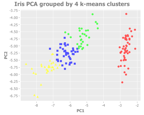
k=4 certainly looks as defensible as k=3, just visually. What we need here is some sort of concrete way to gauge accuracy.
The most common technique to gauge accuracy of a clustering attempt is the elbow method, where one looks for a sharp turn or "elbow" in the graph of the sum of squared errors (or SSE) for each clustering analysis (or "clusterer"). Let's try that.
Here I map our cluster-analysis process across a range of k all the way up to 10. Then I chart the resulting SSEs.
(let [clusterers (map #(mlc/clusterer-info
                        (doto (mlc/make-clusterer :k-means {:number-clusters %})
                          (.buildClusterer (mld/make-dataset
                                            "Fisher's Irises"
                                            [:sepal-length :sepal-width
                                             :petal-length :petal-width]
                                            (i/to-vect (i/sel iris :cols
                                                              (range 4)))))))
                      (range 1 11))]
  (i/view (incc/line-chart (map :number-clusters clusterers)
                           (map :squared-error clusterers)
                           :title "Fisher's irises: SSE by selection of k"
                           :x-label "Number of clusters, k"
                           :y-label "Within-cluster sum of squared errors")))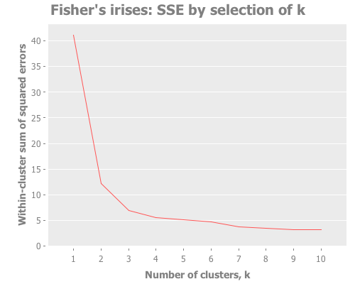
It looks like in the case of the iris data, the "elbow" technique is informative, but leaves us with unanswered questions. There's an elbow at both 2 and 3, and maybe even 4. With this technique we're able to reject k>4 and focus on k=2, k=3, and k=4, but I want more certainty. I would feel more comfortable with something numerically-based to base my conclusions on. Wouldn't you?
Well, that's precisely what Sugar & James provide. They propose calculating the distortion in each clustering analysis, and then looking at the change or 'jump' in distortion from one k to the next. I've created the following functions to do just that.
First, they calculate the 'distortion' for each cluster analysis given k. This means raising the squared error, which we already know, to a negative power that we can manipulate but generally set to one-half of the number of parameters in our data set. Since we want to look at this value across a range of k values, this function applies that calculation to each k-means clusterer in a seq of clusterers:
(defn assoc-distortions
  "Given a number `transformation-power-y` and a seq of maps
  `clusterers`, where each map describes a k-means clusterer, return a
  seq of maps describing the same clusterers, now with key :distortion
  mapped to the value of the cluster analysis' squared error raised to
  the negative `transformation-power-y`.

  Based on Sugar & James' paper at
  http://www-bcf.usc.edu/~gareth/research/ratedist.pdf which defines
  distortion (denoted d[hat][sub k]) for a given k as the mean squared error when covariance
  is the identity matrix. This distortion is then transformed by
  raising it to the negative of the transformation power y, which is
  generally set to the number of attributes divided by two."
  [clusterers transformation-power-y]
  (map #(assoc % :distortion (Math/pow (:squared-error %) (- transformation-power-y)))
       clusterers))
Once you know the distortions, Sugar & James write, you calculate the change in those transformed distortions as one changes k. They call this the "jump", which we calculate by walking our seq of clusterers in a pairwise fashion using partition. Notice that we prepend a dummy clusterer ({:distortion 0}) so that we can calculate a jump for k=1.
(defn assoc-jumps
  "Given a seq of maps `clusterers` each describing a k-means analysis
  including the transformed :distortion of that analysis, returns a
  sequence of maps 'updated' with the calculated jumps in transformed
  distortions.

  Based on Sugar & James' paper at
  http://www-bcf.usc.edu/~gareth/research/ratedist.pdf which defines
  the jump for a given k (denoted J[sub k]) as simply the transformed distortion for k
  minus the transformed distortion for k-1."
  [clusterers]
  (map (fn [[a b]] (assoc b :jump (- (:distortion b) (:distortion a))))
       (partition 2 1 (conj clusterers {:distortion 0}))))
Note that if you ignore the preposterously long-winded docstrings in those two functions, the code itself is rather concise. Powerful mathematical concepts don't have to be complex.
Let's put these distortion and jump tools to work. I want to see them plotted across a selection of k values for our iris data. We also need to try out some different values for the transformation power, Y. (Notice that this turns clustering from a one-dimensional problem of selecting k into a two-dimensional problem of evaluating different combinations of Y and k.) To do that, let's graph the distortion jumps for different values of k across three selections of Y.
(let [clusterers (map #(mlc/clusterer-info
(doto (mlc/make-clusterer :k-means {:number-clusters %})
(.buildClusterer (mld/make-dataset
"Fisher's Irises"
[:sepal-length :sepal-width
:petal-length :petal-width]
(i/to-vect (i/sel iris :cols (range 4)))))))
(range 1 11))]
;; k from 1 to 10 using transformation power of 2/3:
(i/view (incc/line-chart (map :number-clusters (assoc-jumps (assoc-distortions clusterers (/ 2 3))))
(map :jump (assoc-jumps (assoc-distortions clusterers (/ 2 3))))
:title "Fisher's irises: Jumps according to k, with y=2/3 [Figure 5a]"
:x-label "Number of clusters, k"
:y-label "Jumps in transformed distortions, J"))
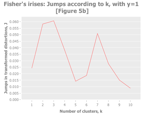
;; k from 1 to 10 using transformation power of 1:
(i/view (incc/line-chart (map :number-clusters (assoc-jumps (assoc-distortions clusterers 1)))
(map :jump (assoc-jumps (assoc-distortions clusterers 1)))
:title "Fisher's irises: Jumps according to k, with y=1 [Figure 5b]"
:x-label "Number of clusters, k"
:y-label "Jumps in transformed distortions, J"))
;; k from 1 to 10 using transformation power of 2:
(i/view (incc/line-chart (map :number-clusters (assoc-jumps (assoc-distortions clusterers 2)))
(map :jump (assoc-jumps (assoc-distortions clusterers 2)))
:title "Fisher's irises: Jumps according to k, with y=2 (p/2) [Figure 5b]"
:x-label "Number of clusters, k"
:y-label "Jumps in transformed distortions, J")))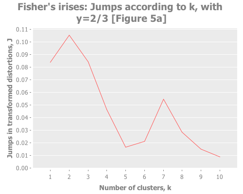
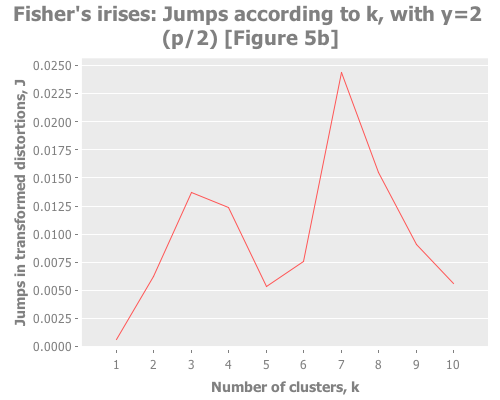
Sugar and James use Y=1 and Y=2/3, and I added Y=2 to see performance of the default recommendation of 1/2 of the number of parameters. Their choice seems based on trial and error:
[Various theoretical reasons and observations] suggest that the further the cluster distributions are from Normal, the smaller the transformation power should be. However, it is not obvious how to choose the optimal value of Y.
...
When squared error distortion is used and strong correlations exist between dimensions, values of Y somewhat less that p = 2 may produce superior results... Empirically, a promising approach involves estimating the “effective” number of dimensions in the data and transforming accordingly. For example, the iris data is four-dimensional which suggests using Y = 2. However, several of the variables are highly correlated. As a result, the effective dimension of this data set is closer to 2, implying that a transformation power near Y = 1 may be more appropriate.
With that understanding, what do these three graphs show? With Y=2, I see a clear spike at k=7 and a secondary spike at k=3. With Y=1, the spike at 7 is greatly diminished, and k=3 barely edges out k=2. With Y=2/3, k=2 is the clear winner. (Your results may vary based on WEKA seeding. More on this in future installments.) You may find it interesting to run these again with dramatically higher maximum k.
Taking the authors' recommendations on selecting a transformation power, I would interpret these results (were I ignorant of the actual number of classes and refused to do any deeper analysis) as suggesting either 2, 3, or 7 clusters. Sugar and James note that either 2 or 3 is a reasonable interpretation of the data given its known classes. I would suggest that k=7 is leaning into overfitting territory given the number of samples per cluster (~21 rather than ~50), but would be a reasonable path to investigate (again, if I were ignorant of the true classes).
Overall, examining jumps in distortion seems like a relatively robust method for this particular data set. Looking at other example data sets can show us more dramatically how this method is superior to the elbow method. We'll do that in part 2.
Also, Part Three.