Title2

SVM.md

Support Vector Machines (SVM)

Support Vector Machine (SVM) é um classificador formalmente definido pela separação de um hiperplano. Em outras palavras, dado um prévio conjunto de dados já classificado (aprendizado supervisionado), o algoritmo retorna um hiperplano ideal que categoriza novos exemplos.

Considere o seguinte problema:

Para um conjunto de pontos 2D que pertencem a duas classes distintas, encontre uma linha reta que separe os pontos de acordo com sua classe.

In the above picture you can see that there exists multiple lines that offer a solution to the problem. Is any of them better than the others? We can intuitively define a criterion to estimate the worth of the lines:

A line is bad if it passes too close to the points because it will be noise sensitive and it will not generalize correctly. Therefore, our goal should be to find the line passing as far as possible from all points.

Then, the operation of the SVM algorithm is based on finding the hyperplane that gives the largest minimum distance to the training examples. Twice, this distance receives the important name of margin within SVM’s theory. Therefore, the optimal separating hyperplane maximizes the margin of the training data.

Nota-se que o objetivo do SVM em um espaço bidimensional é emcontrar uma linha. Porém em um espaço tridimensional o objetivo é encontrar planos e para casos de espaço com mais de três dimensões, o objetivo é encontrar hiperplanos.

Os elementos de cada classe mais próximos da "linha" ótima (destacados na imagem anterior) são chamados de Support Vectors e são utilizados pelo classificador do SVM para fazer uma comparação entre a sua posição e a posição do elemento a ser classificado. Para que isso seja possível, o algoritmo de treinamento do SVM utiliza técnicas de otimização. Uma dessas técnicas é a Sequential minimal optimization (SMO).

O algoritmo do SVM, tanto na aprendizagem como na classificação, ainda é capaz de tratar casos de conjunto de elementos não-linearmente separáveis. Para isso, ele faz o uso de uma função de Kernel, ao invés dos produtos utilizados nas equações para a multiplicação dos vetores de características de dois elementos. Caso o problema ainda assim não seja resolvido, são utilizadas variáveis de folga, fazendo com que a reta de separação seja flexível (SEMOLINI, 2002).

A utilização de uma função de Kernel,$K(x,x')$ tem como objetivo mapear os elementros em um novo espaço com o número de dimensões muito maior do que as do espaço original. Com isso, os elementos podem se tornar linearmente separáveis, já que suas posições no novo espaço são diferentes das no espaço original, possibilitando a definição de um hiperplano que separe os elementos de diferentes classes (HAN e KAMBER, 2006).

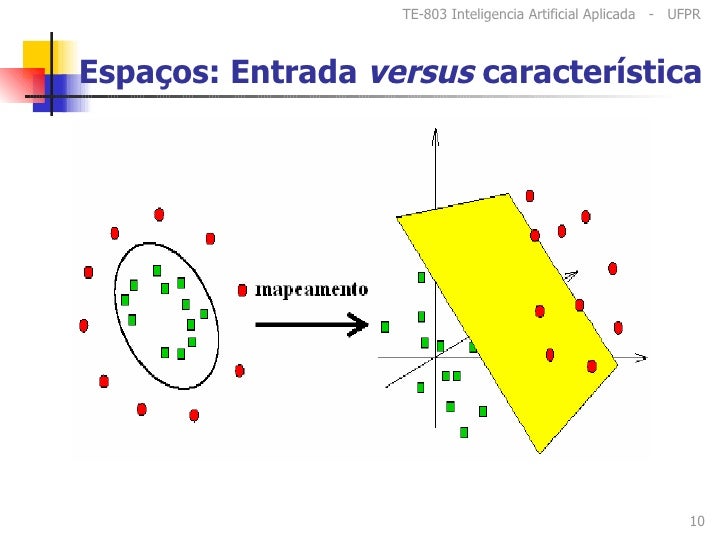
A figura acima ilustra a aplicação de uma função de Kernel, em elementos inicialmente mapeados em um espaço com $m$ dimensões os re-mapeando em um novo espaço com $M$ ‬dimensões onde $M \gt\gt m$ ( SEMOLINI, 2002).

Seque três funções de Kernel mais comuns utilizadas em SVM :

• Função de Base Radial (RBF)
• Função Polinomial
• Perceptron

Sequential minimal optimization (SMO)

Sequential minimal optimization (SMO) is an algorithm for solving the optimization problem which arises during the training of support vector machines. It was invented by John Platt in 1998 at Microsoft Research.[1] SMO is widely used for training support vector machines and is implemented by the popular LIBSVM tool.[2][3] The publication of the SMO algorithm in 1998 has generated a lot of excitement in the SVM community, as previously available methods for SVM training were much more complex and required expensive third-party QP solvers

Consider a binary classification problem with a dataset $(x1, y1), ..., (xn, yn)$, where $xi$ is an input vector and $yi ∈ {-1, +1}$ is a binary label corresponding to it. A soft-margin support vector machine is trained by solving a quadratic programming problem, which is expressed in the dual form as follows:

$\max_{\alpha} \sum_{i=1}^n \alpha_i - \frac12 \sum_{i=1}^n \sum_{j=1}^n y_i y_j K(x_i, x_j) \alpha_i \alpha_j$,

subject to:

$0 \leq \alpha_i \leq C, \quad \mbox{ for } i=1, 2, \ldots, n$,

$\sum_{i=1}^n y_i \alpha_i = 0$

where $C$ is an SVM hyperparameter and $K(xi, xj)$ is the kernel function, both supplied by the user; and the variables $\alpha_i$ are Lagrange multipliers.

Algorithm

SMO is an iterative algorithm for solving the optimization problem described above. SMO breaks this problem into a series of smallest possible sub-problems, which are then solved analytically. Because of the linear equality constraint involving the Lagrange multipliers $\alpha_i$, the smallest possible problem involves two such multipliers. Then, for any two multipliers $\alpha_1$ and $\alpha_2$, the constraints are reduced to:

$0 \leq \alpha_1, \alpha_2 \leq C$,

$y_1 \alpha_1 + y_2 \alpha_2 = k$,

and this reduced problem can be solved analytically: one needs to find a minimum of a one-dimensional quadratic function. k is the sum over the rest of terms in the equality constraint, which is fixed in each iteration.

The algorithm proceeds as follows:

1. Find a Lagrange multiplier $\alpha_1$ that violates the Karush–Kuhn–Tucker (KKT) conditions for the optimization problem.
2. Pick a second multiplier $\alpha_2$ and optimize the pair ($\alpha_1,\alpha_2$).
3. Repeat steps 1 and 2 until convergence.

When all the Lagrange multipliers satisfy the KKT conditions (within a user-defined tolerance), the problem has been solved. Although this algorithm is guaranteed to converge, heuristics are used to choose the pair of multipliers so as to accelerate the rate of convergence.

Radio Basis Function Kernel (RBFKernel)

In machine learning, the (Gaussian) radial basis function kernel, or RBF kernel, is a popular kernel function used in support vector machine classification.[1]

The RBF kernel on two samples $x$ and $x'$, represented as feature vectors in some input space, is defined as[2]

$K(\mathbf{x}, \mathbf{x'}) = \exp\left(-\frac{||\mathbf{x} - \mathbf{x'}||_2^2}{2\sigma^2}\right)$

$\textstyle||\mathbf{x} - \mathbf{x'}||_2^2$ may be recognized as the squared Euclidean distance between the two feature vectors. $\sigma$ is a free parameter. An equivalent, but simpler, definition involves a parameter $\textstyle\gamma = -\tfrac{1}{2\sigma^2}$:

$K(\mathbf{x}, \mathbf{x'}) = \exp(\gamma||\mathbf{x} - \mathbf{x'}||_2^2)$

Since the value of the RBF kernel decreases with distance and ranges between zero (in the limit) and one (when $x = x'$), it has a ready interpretation as a similarity measure.[2] The feature space of the kernel has an infinite number of dimensions; for $\sigma = 1$, its expansion is:[3]

$\exp\left(-\frac{1}{2}||\mathbf{x} - \mathbf{x'}||2^2\right) = \sum{j=0}^\infty \frac{(\mathbf{x}^\top \mathbf{x'})^j}{j!} \exp\left(-\frac{1}{2}||\mathbf{x}||_2^2\right) \exp\left(-\frac{1}{2}||\mathbf{x'}||_2^2\right)$

Referências

• OpenCV - Introduction to SVM

• Wikipedia - Radial basis function kernel

• Wikipedia - Support Vector Machine

• Wikipedia - Sequential Minimal Optimization

Hola soy nuevo

Es La mejor aplicación del mundo