Generalized Voronoi “tesselation”

voronoi.md

Generalized Voronoi “tesselation”: variation on a theme (AoC 2018, Day 6)

The point of this vignette is to introduce a simple notion of a generalized Voronoi tesselation (in the context of Day 6), and to illustrate how they can be implemented succinctly with tensors.

Day 6, abstractly

A common procedure can be applied to solve both parts of the Day 6 puzzle:

1. Compute a suitable generalized Voronoi tesselation.

2. Filter the tesselation (by a predicate function).

3. Aggregate the filtered result (by sum or max).

Each step corresponds to a (pure) function. The solution amounts to composing the functions and applying it to the given set of points.

What do I mean by “generalized Voronoi tesselation?” Well, in addition to the dependence on a metric (typically, “Manhattan” or Euclidean), a Voronoi tesselation has another degree of freedom: the tesselation function itself. Typically, this is described as the function that “colors” each locations by the nearest point. But I think a more edifying notion is the following:

• A (generalized) tesselation is a function sending the tensor of distances to the points to a value of some type a (which is usually Bool or Int).

Using pseudo-Haskell, we can thus describe a Voronoi tesselation as a function of the following type:

voronoi :: Metric -> Tesselation -> [Point] -> a

where Point is a type for the coordinates (say, [[Double]]), and Metric and Tesselation are function types:

type Metric = Point -> Point -> Double
type Tesselation = Tensor -> a

Here Tensor is a type for rank 3 tensors, which could be faked by [[[Double]]]. (Why rank 3? That will be explained below.)

Why not Haskell?

Truth is, despite the talk about types, I will not be implementing the above ideas in Haskell. Instead, I will use R, a dynamically typed language, for the following reasons:

• I don’t know Haskell well enough to implement the ideas below. (Also, ideally one should use dependent types. There is a simulacrum of this in the higher-order function map_dbl(), see below.)

• It will be useful to visualize the Voronoi “tesselations” along the way. R is an excellent language for that.

• It is possible to write (non-idiomatic) R in a functional, point-free style, which is faithful to the functional plan outlined above.

A Voronoi tesselation function

Rather than implementing one of the known algorithms, I’ll just do it from scratch. Of course, the implementation that follows, while straightforward, is not efficient. But it’s good enough for the puzzle. It is also an illustration of “thinking in arrays.” As a style of programming, this has its roots in APL; as a mathematical method, it goes back to Hermann Grassmann, at least.

Some higher order functions

As I mentioned, R, despite taking inspiration from Scheme, is not a functional language. But we can pretend that it is by rolling our own higher-order functions for working with tensors. The package gestalt (by yours truly) provides the quasiquotation-enabled lambda constructors fn(), fn_() and the (forward) composition operator %>>>%.

library(gestalt)

fmap_col <- fn_(f ~ fn(xs, ... ~ apply(xs, 2, !!f, ...)))
fmap_mtx <- fn_(f ~ fn(xs, ... ~ apply(xs, 1:2, !!f, ...)))

map_dbl <- fn(xs, f, ... = , .dim = 1 ~ {
  vapply(xs, f, ..., FUN.VALUE = array(NA_real_, .dim))
})

(Remark: The funny looking !! is an unquoting operator. I use it to force eagar evaluation.)

Voronoi “tesselations”

The function voronoi() below has the signature of our fantasy voronoi, above. It takes a 2-by-2 matrix of (coordinates of) points, a metric (default “Manhattan”), a tesselation function (default “matrix-wise argmin,” aka “color by nearest point”), and returns the tesselated matrix, wrapped as an object that also records the points. (Why do we keep the points? So that we may plot them!)

library(dub)  # Provides %<<-% (unpacking assignment)

voronoi <- local({
  normalize <- fmap_col(fn(. ~ . - min(.) + 1))
  shape <- fmap_col(max)
  as_voronoi <- list %>>>% `class<-`(c("Voronoi", "matrix"))
    
  fn(pts, metric = L1_metric, tesselate = argmin_mtx ~ {
    pts <- normalize(pts)
    (w : h) %<<-% shape(pts)
    dists <- map_dbl(rows(pts), metric(w, h), .dim = c(h, w))
    as_voronoi(raster = tesselate(dists), points = pts)
  })
})

# Helper function to transpose a matrix to a list of its rows
rows <- partial(apply, MARGIN = 1, FUN = as.list)

The way the function voronoi() works is straightforward. It’s a sequence of three tensor transformations:

1. Starting with the matrix of coordinates, we normalize them by shifting the origin to the bounding box of the points. This is okay because any reasonable notion of “tesselation” should be translation invariant. The subsequent code is less noisy under the assumption of normalized coordinates.

2. From the matrix of coordinates, we then compute a rank 3 tensor (a 3-dimensional array) of distances from locations in the bounded box—computed by metric(w, h)—to the given points. This is dists. Its first two dimensions are given by the size of the bounding box, while the third is indexed by the set of points (in their given order).

3. Lastly, the tensor dists is “tesselated”: the function tesselate() maps over the third dimension of dists to return a matrix with dimensions of the bounding box.

Metrics

We define metrics via a constructor, as_metric(), that turns a formula for a metric into a function of a point.

as_metric <- local({
  locations <- fn(w, h ~ {
    locs <- seq_len(w * h) - 1
    array(c(x = locs %/% h + 1, y = locs %% h + 1), c(h, w, 2), nms)
  })
  nms <- list(NULL, NULL, c("x", "y"))
  
  fn_(fml ~ fn(w, h, loc = locations(w, h) ~ fn(!!fml)))
})

L1_metric <- as_metric(
  . ~ abs(.[["x"]] - loc[, , "x"]) + abs(.[["y"]] - loc[, , "y"])
)

For example, the Euclidean metric would be constructed thus:

L2_metric <- as_metric(
  . ~ sqrt((.[["x"]] - loc[, , "x"])^2 + (.[["y"]] - loc[, , "y"])^2)
)

Ordinary tesselation

The ordinary Voronoi tesselation is computed by finding, for each location, the closest point. The jargon for this is “arg-min” (for “minimizing argument”). The only noteworthy point here is that arg-min has to be lifted by “fmap” in order that it can map over a (rank 3) tensor.

argmin <- fn(x, break_tie = 0L ~ {
  i <- which(x == min(x))
  if (length(i) == 1) i else break_tie
})

argmin_mtx <- fmap_mtx(argmin)

Visualizing Voronoi tesselations

The way plotting of objects works in R is that you define a “print” method that plots to the graphics device. Since the function voronoi() returns an object of (S3) class "Voronoi", we need to implement a function named print.Voronoi. The details are straightforward and uninteresting. The only thing to note is that I’ve added an option to show the points, by toggling the argument show_points (default TRUE).

print.Voronoi <- local({
  flip <- {.[nrow(.):1, ]} %>>>% t
  
  overlay_points <- fn(v ~ {
    (h : w) %<<-% dim(v$raster)
    for (i in seq_len(nrow(v$points))) {
      (x : y) %<<-% v$points[i, ]
      v$raster[y, segment(x, w)] <- 0
      v$raster[segment(y, h), x] <- 0
    }
    v
  })
  segment <- fn(x, n, side = seq.int(-1, 1) ~ {
    xs <- x + side
    xs[xs >= 1 & xs <= n]
  })
  
  fn(x, col = c("black", rainbow(64)), show_points = TRUE, ... ~ {
    if (show_points)
      x <- overlay_points(x)
    image(flip(x$raster), xaxt = "n", yaxt = "n", col = col, ...)
  })
})

A test visualization

Here’s the example from the problem:

pts_test <- c(1, 1,
              1, 6,
              8, 3,
              3, 4,
              5, 5,
              8, 9)
pts_test <- matrix(pts_test, ncol = 2, byrow = TRUE)
colnames(pts_test) <- c("x", "y")

pts_test

#>      x y
#> [1,] 1 1
#> [2,] 1 6
#> [3,] 8 3
#> [4,] 3 4
#> [5,] 5 5
#> [6,] 8 9

The claim is that the Voronoi tesselation should look like this:

aaaaa.cccc
aAaaa.cccc
aaaddecccc
aadddeccCc
..dDdeeccc
bb.deEeecc
bBb.eeee..
bbb.eeefff
bbb.eeffff
bbb.ffffFf

Indeed, it does:

print(voronoi(pts_test), show_points = FALSE)

(I’ve turned off the points, because at such a low resolution, they occupy a large portion of the raster.)

Visualizing the Voronoi tesselation

First, here’s a peek at the dataset from the problem:

pts <- read.csv("../data/input-06", header = FALSE, col.names = c("x", "y"))
head(pts)

#>     x   y
#> 1  78 335
#> 2  74 309
#> 3 277  44
#> 4 178 286
#> 5 239 252
#> 6 118 354

Here’s what the Voronoi tesselation looks like with the Manhattan metric (the black boundary streaks are the locations equidistant to two or more points):

voronoi(pts)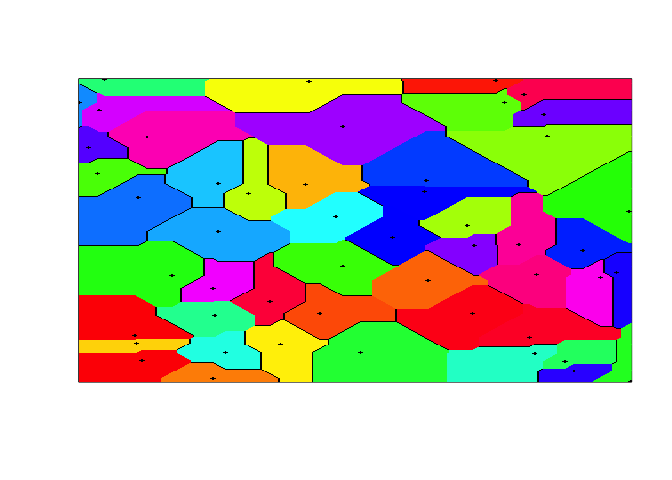

And in the Euclidean metric:

voronoi(pts, metric = L2_metric)

These pictures seem consistent with the illustrations on Wikipedia. I take that as (informal) corroboration of the correctness of the function voronoi().

Solution to Part 1

What is the size of the largest area that isn’t infinite?

The problem is to find the area of the largest bounded cell in the Voronoi tesselation of the points. Let’s call the function that will do this max_finite_area().

So far, we have completed the function for the first step. Recall that the remaining steps are:

2. Filter the tesselation (by a predicate function).

3. Aggregate the filtered result (by sum or max).

max_finite_area() will be a composition of voronoi() and the functions for these two steps. Here’s an implementation following that prescription:

max_finite_area <- (
  voronoi
  %>>>% filter: {.$raster[is_bounded(.$raster)]}
  %>>>% aggregate: (table %>>>% max)
)

The tags filter and aggregate are simply annotations (names). The filter component is a function that maps ., a placeholder for the output of the preceding function, to a filtering of the raster of the tesselation. The aggregate component then tabulates the values and finds the max among those.

The predicate function is_bounded() finds the complement of the points whose Voronoi cells are unbounded—these are the ones that meet the boundary of the bounding box (proof?):

is_bounded <- fn(raster ~ {
  boundary <- c(
    raster[1, ],
    raster[nrow(raster), ],
    raster[, 1],
    raster[, ncol(raster)]
  )
  !(raster %in% c(0, boundary))
})

A quick verification of the claim about the example dataset:

stopifnot(max_finite_area(pts_test) == 17)

And now the answer to Part 1:

stopifnot(max_finite_area(pts) == 4887)

Solution to Part 2

What is the size of the region containing all locations which have a total distance to all given coordinates of less than 10000?

As I mentioned at the very outset, the form of the solution of this part is identical, mutatis mutandis, to that in the previous part. The required changes are evident:

• Instead of finding the nearest point to a location, we need to add the distances from a location to all the points. The tesselation function argmin_mtx should be switched to sum, or rather its tensor fmap’d version, fmap_mtx(sum).

• We filter the resulting tesselation by applying a cutoff.

• Since we want to compute the size of the region, we aggregate by taking a sum of the filtered tesselation points.

Applying this literally, we get the following:

sum_mtx <- fmap_mtx(sum)

bounded_area <- (
  voronoi(tesselate = sum_mtx)
  %>>>% filter: {.$raster < 1e4}
  %>>>% aggregate: sum
)

Let’s verify this against the example dataset. The claim is that when the total distance to all given coordinates is capped at 32, the resulting region of points should look like this:

..........
.A........
..........
...###..C.
..#D###...
..###E#...
.B.###....
..........
..........
........F.

Indeed, it does:

print(voronoi(pts_test, tesselate = fn(. ~ sum_mtx(.) < 32)),
      show_points = FALSE)

Here is the answer to Part 2:

stopifnot(bounded_area(pts) == 34096)

For the tesselation function sum_mtx(), the generalized Voronoi tesselation is a “topographic” map whose contour lines correspond to locations of a constant total distance to all given points:

voronoi(pts, tesselate = sum_mtx)

Likewise, the region of points whose size yields the answer to this part of the puzzle is a generalized Voronoi tesselation. The tesselation function is the sum-cutoff predicate:

voronoi(pts, tesselate = fn(. ~ sum_mtx(.) < 1e4))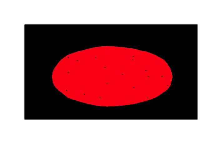

Every one of these images represent a generalized Voronoi tesselation. Their visual diversity reflects the richness of these functions.