Copy of https://rentry.org/llm-training on 2023-10-10

llm-training.md

-> <-

The Novice's LLM Training Guide

->Written by Alpin<- ->Inspired by /hdg/'s LoRA train rentry<-

The Table of Content on rentry is terrible, so I'll be linking to the different main sections here:

• Training from Scratch
• Native Fine-Tuning
• LoRA
• QLoRA
• Training Hyperparameters
• Interpreting the Learning Curves

---

[TOC2]

---

The Basics

A modern Large Language Model (LLM) is trained using the Transformers library, which leverages the power of the Transformer network architecture. This architecture has revolutionized the field of natural language processing and is widely adopted for training LLMs. Python, a high-level programming language, is commonly used for implementing LLMs, making them more accessible and easier to comprehend compared to lower-level frameworks such as OpenXLA's IREE or GGML. The intuitive nature of Python allows researchers and developers to focus on the logic and algorithms of the model without getting caught up in intricate implementation details.

This rentry won't go over pre-training LLMs (training from scratch), but rather fine-tuning and low-rank adaptation (LoRA) methods. Pre-training is prohibitively expensive, and if you have the compute for it, you're likely smart enough not to need this rentry at all.

Using LLMs

There are quite a few guides for using LLMs either locally on your PC or using a cloud computing service (often for a fee). Transformers models hosted on HuggingFace are the easiest to run, and several UIs offer inference for them:

• Text Generation Web UI
• KoboldAI
• llama.cpp

The compute requirement for the model can be calculated by multiplying the amount of space your model occupies on your hard disk by a factor of 1.2. Source: Transformer Math 101

For instance, let's consider the LLaMA 7B model, which occupies approximately 13.5 GB of storage space. To estimate the required VRAM for inference, we can multiply this value by 1.2, resulting in approximately 16.2 GB. This additional 20% accounts for overhead and the memory necessary for context token processing. It's important to note that the overhead will vary significantly based on the model's context size. The estimation assumes a model with an n_ctx (context size) of 2048.

In traditional attention mechanisms, the memory usage for context scales quadratically. However, newer techniques such as Flash Attention allow for linear scaling, reducing the memory footprint.

Further reading:

• Transformer Inference Arithmetic

The Transformer architecture

It's always good practice to have an understanding of what you're working with, though it's not strictly necessary for fine-tuning purposes, since you'll be running scripts that call the Transformers library's Trainer class.

The best source is, of course, the Attention Is All You Need paper. It introduced the Transformer architecture and is a profoundly important paper to read through. You might, however, need to read these first, since the authors assume you already have a basic grasp of neural networks. I recommend reading these in order:

• Deep Learning in Neural Networks: an Overview
• An Introduction to Convolutional Neural Networks
• Recurrent Neural Networks (RNNs): A gentle Introduction and Overview

!!!note Paper too hard to read? You're not alone. Academics tend to intentionally obfuscate their papers. You can always look for blog posts or articles on each topic, where they tend to provide easy to digest explanations. One great resource is HuggingFace blogposts.

---

Training Basics

There's essentially three (3) approaches to training LLMs: pre-training, fine-tuning, and LoRA.

Pre-training

Pre-training involves several steps. First, a massive dataset of text data, often in terabytes, is gathered. Next, a model architecture is chosen or created specifically for the task at hand. Additionally, a tokenizer is trained to appropriately handle the data, ensuring that it can efficiently encode and decode text. The dataset is then pre-processed using the tokenizer's vocabulary, converting the raw text into a format suitable for training the model. This step involves tokenizing the text, mapping tokens to their corresponding IDs, and incorporating any necessary special tokens or attention masks. Once the dataset is pre-processed, it is ready to be used for the pre-training phase.

During pre-training, the model learns to predict the next word in a sentence or to fill in missing words by utilizing the vast amount of data available. This process involves optimizing the model's parameters through an iterative training procedure that maximizes the likelihood of generating the correct word or sequence of words given the context.

To accomplish this, the pre-training phase typically employs a variant of the self-supervised learning technique. The model is presented with partially masked input sequences, where certain tokens are intentionally hidden, and it must predict those missing tokens based on the surrounding context. By training on massive amounts of data in this manner, the model gradually develops a rich understanding of language patterns, grammar, and semantic relationships. This specific approach is for Masked Language Modeling. The most commonly used method, however, is Causal Language Modeling. Unlike masked language modeling, where certain tokens are masked and the model predicts those missing tokens, causal language modeling focuses on predicting the next word in a sentence given the preceding context.

This initial pre-training phase aims to capture general language knowledge, making the model a proficient language encoder. But, unsurprisingly, it lacks specific knowledge about a particular task or domain. To bridge this gap, a subsequent fine-tuning phase follows pre-training.

Fine-tuning

After the initial pre-training phase, where the model learns general language knowledge, fine-tuning allows us to specialize the model's capabilities and optimize its performance on a narrower, task-specific dataset.

The process of fine-tuning involves several key steps. Firstly, a task-specific dataset is gathered, consisting of labeled examples relevant to the desired task. For example, if the task is instruct-tuning, a dataset of instruction-response pair is gathered. The fine-tuning dataset size is significantly smaller than the sets typically used for pre-training.

Next, the pre-trained model is initialized with its previously learned parameters and architecture. The model is then trained on the task-specific dataset, optimizing its parameters to minimize a task-specific loss function. This loss function quantifies the difference between the model's predictions and the true labels provided in the dataset.

During fine-tuning, the parameters of the pre-trained model are adjusted using gradient-based optimization algorithms such as stochastic gradient descent (SGD) or Adam. The gradients are computed by backpropagating the loss through the model's layers, allowing the model to learn from its mistakes and update its parameters accordingly.

To enhance the fine-tuning process, additional techniques can be employed, such as learning rate scheduling, regularization methods like dropout or weight decay, or early stopping to prevent overfitting. These techniques help optimize the model's generalization and prevent it from memorizing the training dataset too closely.

Low-Rank Adaptation (LoRA)

Fine-tuning is computationally expensive, requiring hundreds of GBs of VRAM for training multi-billion parameter models. To solve this specific problem, a new method was proposed: Low-Rank Adaptation. Compared to fine-tuning OPT-175B with Adam, LoRA can reduce the number of trainable parameters by 10,000 times and the GPU memory requirements by over 3 times. Refer to the paper LoRA: Low-Rank Adaptation of Large Language Models and the HuggingFace PEFT: Parameter-Efficient Fine-Tuning of Billion-Scale Models on Low-Resource Hardware blog post.

A 3x memory requirement reduction is still in the realm of unfeasible for the average consumer. Fortunately, a new LoRA training method was introduced very recently: Quantized Low-Rank Adaptation (QLoRA). It leverages the bitsandbytes library for on-the-fly and near-lossless quantization of language models and applies it to the LoRA training procedure. This results in massive reductions in memory requirement - enabling the training of models as large as 65 billion parameters on 2x NVIDIA RTX 3090s! For comparison, you would normally require over 16x A100-80GB GPUs for fine-tuning a model of that size class; the associated cost would be tremendous.

This next sections of this rentry will focus on the fine-tuning and LoRA/QLoRA methods.

---

Training from Scratch

Weights and Biases very recently released a whitepaper guide for training LLMs from scratch. You can read it here.

Native Fine-tuning

As explained earlier, fine-tuning can be expensive, depending on the model size you choose. You typically want at least 6B/7B parameters. We'll go through some options for acquiring training compute.

Training Compute

Depending on your model and dataset size, the memory requirement will vary. You can, once again, refer to EleutherAI's Transformer Math 101 blog post for detailed, but easy to understand, calculations.

You will want to fine-tune a model of at least the 6B/7B class. Some popular options are GPT-J 6B, LLaMA 7B, Pythia-6.9B DeDuped, etc. This size class typically requires memory in the 160~192GB range. Your options, essentially, boil down to:

• Renting GPUs from cloud services; e.g. Runpod, VastAI, Lambdalabs, and Amazon AWS Sagemaker. Out of the four examples, VastAI is the cheapest (but also the least reliable), while Amazon Sagemaker is the most expensive. I recommend using either Runpod or Lambdalabs.

• Using Google's TPU Research Cloud You can apply for free access to the Google TRC program and potentially receive up to 110 TPU machines. Keep in mind that TPUs are significantly different, architecture-wise, from GPUs; you will need to learn how they work first before committing to your 30-day free TRC plan. Fortunately, google provides free access to TPUs (albeit weak ones) via Google Colaboratory. There are also libraries and guides made for fine-tuning LLMs on TPUs. The Mesh Transformers JAX repository has a guide for fine-tuning GPT-J models on TRC, and EasyLM provides an easy way to pre-train, fine-tune and evaluate language models on both TPUs and GPUs.

• Know a guy who knows a guy. Maybe one of your friends knows someone with access to a supercomputer. Wouldn't that be cool?

Gathering a Dataset

Dataset gathering is, without a doubt, the most important part of your fine-tuning journey. Both quality and quantity matter - though quality is more important.

First, think about what you want the fine-tuned model to do. Write stories? Role-play? Write your emails for you? Maybe you want to create your AI waifubot. For the purposes of this rentry, let's assume you want to train a chat & roleplaying model, like Pygmalion. You'll want to gather a dataset of conversations. Specifically, conversations in the style of internet RP. The gathering part might be quite challenging; you'll have to figure that out yourself :D

Dataset structure

You'll want to outline a structure for your dataset. Essentially, you want:

• Data Diversity: You don't want your models to only do one very specific task. In our assumed use-case, we're training a chat model, but this doesn't mean the data would only be about one specific type of chat/RP. You will want to diversify your training samples, include all kinds of scenarios so that your model can learn how to generate outputs for various types of input.

• Dataset size: Unlike LoRAs or Soft Prompts, you'll want a relatively large amount of data. This is, of course, not on the same level as pre-training datasets. As a rule of thumb, make sure you have at least 100 MiB of data for your fine-tune. It's incredibly difficult to overtrain your model, so it's always a good idea to stack more data.

• Dataset quality: The quality of your data is incredibly important. You want your dataset to reflect how the model should turn out. If you feed it garbage, it'll spit out garbage.

Processing the raw dataset

You may have a bunch of text data now. Before you continue, you will want to parse them into a suitable format for pre-processing. Let's assume your dataset is in one of these conditions:

HTML

You might have HTML files if you scraped your data from websites. In that case, your priority will be pulling data out of the HTML elements. If you're not right in the head, you'll try and use pure RegEx to do this. This is extremely inefficient, so thankfully there are libraries that handle this issue. You can use the Beautiful Soup Python library to help you with this. You can read the documentation for it, but it's generally used this way:

from bs4 import BeautifulSoup

# HTML content to be parsed
html_content = '''
<html>
<head>
<title>Example HTML Page</title>
</head>
<body>
<h1>Welcome to the Example Page</h1>
<p>This is a paragraph of text.</p>
<div class="content">
    <h2>Section 1</h2>
    <p>This is the first section.</p>
</div>
<div class="content">
    <h2>Section 2</h2>
    <p>This is the second section.</p>
</div>
</body>
</html>
'''

# Create a BeautifulSoup object
soup = BeautifulSoup(html_content, 'html.parser')

# Extract text from the HTML
text = soup.get_text()

# Print the extracted text
print(text)

You'll have an output like this:

Example HTML Page

Welcome to the Example Page
This is a paragraph of text.
Section 1
This is the first section.
Section 2
This is the second section.

CSV

You could have CSV files if you've obtained your dataset from online open data sources. The easiest way to parse them is using the pandas python library. The basic usage would be:

import pandas as pd

# Read the CSV file
df = pd.read_csv('dataset.csv')

# Extract plaintext from a specific column
column_data = df['column_name'].astype(str)
plaintext = column_data.to_string(index=False)

# Print the extracted plaintext data
print(plaintext)

You'll have to specify the column name.

SQL

This one will be a bit tougher. You can take the sensible approach and use a DB framework such as MariaDB or PostgreSQL to parse the dataset into plaintext, but there are also Python libraries for this purpose; one example is sqlparse. The basic usage is:

>>> import sqlparse

>>> # Split a string containing two SQL statements:
>>> raw = 'select * from foo; select * from bar;'
>>> statements = sqlparse.split(raw)
>>> statements
['select * from foo;', 'select * from bar;']

>>> # Format the first statement and print it out:
>>> first = statements[0]
>>> print(sqlparse.format(first, reindent=True, keyword_case='upper'))
SELECT *
FROM foo;

>>> # Parsing a SQL statement:
>>> parsed = sqlparse.parse('select * from foo')[0]
>>> parsed.tokens
[<DML 'select' at 0x7f22c5e15368>, <Whitespace ' ' at 0x7f22c5e153b0>, <Wildcard '*' … ]
>>>

Clustering the dataset

You can use clustering as an effective tool in achieving data diversity by grouping similar data points together and thus increasing the probability of creating diversity for the fine-tuning dataset. If you have a rather small dataset, you can ignore this step entirely. For absurdly large fine-tune datasets, it's important to apply clustering techniques to isolate unnecessary or noisy data from your overall dataset.

The framing of the clustering problem would be different for each use-case. When you start your data clustering experiments, you'll have to figure out what variables you want to use. There's many ways to cluster data, so you'll have to decide on one that works the best.

The clustering problem is very difficult to implement. You should consider using the K-means clustering techniques from PyTorch.

Minimizing the noise

The best language models are stochastic, which makes it difficult to predict their behaviour, even if the input prompt remains the same. This can, on occasion, result in low-quality and undesirable outputs. You will want to make sure your dataset is cleaned out of unwanted elements. This is doubly important if your data source is synthetic, i.e. generating by GPT-4/3. You might want to truncate or remove the mention of phrases such as "As an AI language model...", "harmful or offensive content...", "...trained by OpenAI...", etc. This script by ehartford is a good filter for this specific task.

Preparing dataset for tokenization

Now, you'll want have to decide how you want to train the model: supervised or unsupervised. For unsupervised training, you'll generally add your dataset to a jsonline file (2048 tokens per line, depending on the base model), and place each sequence inside a text key value. If you're doing supervised training, you'll generally want two keys instead: input and output, though this is can be an arbitrary name. The input would act as the prompt you'll be giving the model, and the output would be what the model is expected to generate when faced with such an input.

Once you're done, save your dataset to a .jsonl file.

Generating train and validation splits

Not all training scripts require doing this, as they usually generate the validation split automatically. Some, however, might require this step (such as the PygmalionAI training code.

As a general rule of thumb, you should split off 0.1% or 0.01% (depending on how large your dataset is) of your data to use as the validation set. Here's a sample code for splitting your dataset:

import random
import argparse
import jsonlines

if __name__ == "__main__":
    parser = argparse.ArgumentParser(description="Split data into training and validation sets.")
    parser.add_argument("--input", type=str, help="Input file to split.")
    parser.add_argument("--split_ratio", type=str, help="Ratio of data to use for training and validation sets in the format 'train_ratio,val_ratio'")
    args = parser.parse_args()

    # Parse the split ratios
    try:
        train_ratio, val_ratio = [float(x) for x in args.split_ratio.split(",")]
    except ValueError:
        print("Invalid split_ratio format. Please use 'train_ratio,val_ratio'")
        exit()

    # Check that the ratios are valid
    if train_ratio <= 0 or val_ratio <= 0:
        print("Invalid ratios. train_ratio and val_ratio must be greater than 0.")
        exit()

    total_ratio = train_ratio + val_ratio

    with jsonlines.open(args.input, 'r') as fin, \
            jsonlines.open("train.jsonl", 'w') as train_out, \
            jsonlines.open("val.jsonl", 'w') as val_out:
        for line in fin:
            r = random.uniform(0, total_ratio)
            if r < train_ratio:
                train_out.write(line)
            else:
                val_out.write(line)

Save this as a python file, and run it with the command python3 foobar.py --input /path/to/dataset.jsonl --split_ratio 0.99,0.01. This should give you two files: train.jsonl and val.jsonl. The validation set is randomly selected from the sequences in the dataset file.

Tokenizing the dataset

Depending on what training code you use, you might not need to do this step. Some, though, require a pre-processed dataset that is converted to Apache PyArrow format. One example is the PygmalionAI training code. The reason for this is typically because the dataset is too big, and you don't want to run the processing step every time you restart a run.

Let's assume you're using the Pygmalion training code. Once you have your train and validation splits, clone the training code git clone https://github.com/PygmalionAI/training-code, install the requirements by running pip install -r requirements.txt inside the cloned directory. Assuming your base model is RedPajama 3B, you'll run:

python3 ./preparation/tokenize_data.py \
  --input-file '/path/to/train.jsonl' \
  --output-file '/path/to/train.arrow' \
  --tokenizer-path 'togethercomputer/RedPajama-INCITE-Base-3B-v1' \
  --max-length 2048

python3 ./preparation/tokenize_data.py \
  --input-file '/path/to/eval.jsonl' \
  --output-file '/path/to/eval.arrow' \
  --tokenizer-path 'togethercomputer/RedPajama-INCITE-Base-3B-v1' \
  --max-length 2048

This will produce two .arrow files in your specified output directory. Keep in mind that tokenized arrow files can take over 5x the amount of disk space jsonline files would. Another thing to note is that the tokenizer script in PygmalionAI training code assumes the prompt and generation keys instead of the more traditional input and output. You can either modify the training code by replacing instances of prompt with input and the same for the generation, or you could change the key names in your dataset instead.

Starting the fine-tune run

You're now ready to start fine-tuning. Let's assume, for the sake of simplicity, that you're fine-tuning RedPajama 3B Base. If you're not on Google TRC, you can use a single A100-80G. Model parallelism is incredibly difficult to get working, so you'll be the most comfortable with a single GPU. You can start a train run with the PygmalionAI code by running this script in the root training-code/ directory:

#!/usr/bin/env bash

export OMP_NUM_THREADS=4
export WANDB_PROJECT="project-name"

OUTPUT_DIR="/data/checkpoints/$WANDB_PROJECT"

MODEL_NAME='EleutherAI/togethercomputer/RedPajama-INCITE-Base-3B-v1'
TRAIN_DATASET="/data/$WANDB_PROJECT/train.arrow"
EVAL_DATASET="/data/$WANDB_PROJECT/eval.arrow"

BSZ=8

accelerate launch \
    './training/hf_trainer.py' \
    --model_name_or_path "$MODEL_NAME" \
    --train_file "$TRAIN_DATASET" \
    --eval_file "$EVAL_DATASET" \
    --output_dir "$OUTPUT_DIR" \
    --report_to "wandb" \
    --do_train --do_eval \
    --ddp_find_unused_parameters false \
    --optim 'adamw_torch_fused' \
    --seed 42 --data_seed 42 \
    --logging_first_step true --logging_steps 1 \
    --dataloader_num_workers 1 \
    --per_device_train_batch_size "$BSZ" --per_device_eval_batch_size "$BSZ" \
    --fp16 true \
    --evaluation_strategy "steps" --eval_steps 128 \
    --save_strategy "steps" --save_steps 128 \
    --save_total_limit 2 \
    --gradient_accumulation_steps 8 \
    --learning_rate 1.0e-5 \
    --lr_scheduler_type "cosine" \
    --warmup_steps 64 \
    --num_train_epochs 1 \
    $@

Explanation of each flag:

• --model_name_or_path: specify the model name (huggingface path) or local directory path.
• --train_file: your pre-processed and tokenized training file.
• --eval_file: your pre-processed and tokenized validation file.
• --output_dir: the output directory for your model checkpoints.
• --report_to: what service to use for real-time logging and reporting of the train run.
• --do_train: perform train.
• --do_eval: perform evaluation using the validation dataset.
• --ddp_find_unused_parameters false: disables distributed data parallel, ensuring all parameters are properly synced during backpropagation.
• --optim what optimizer to use for training.
• --seed and --data_seed: set a seed number for controlling the randomness in the train run, which includes shuffling the data, weight initialization, etc. Setting a seed ensures that good runs are reproducible. Set to -1 for a random number to be used.
• --logging_first_step: only prints logs for the first training step to prevent cluttering the console.
• --dataloader_num_workers: the number of CPU cores to use for loading the datasets.
• --per_device_train_batch_size: the batch size for the training process. Higher means more memory usage.
• --per_device_eval_batch_size: the batch size for the evaluation process. Higher means more memory usage.
• --fp16: the precision to use for training. In this case, float-point 16bits.
• --evaluation_strategy: what strategy to use for evaluation. In this case, evaluated based on the specified number of steps.
• --save_strategy: what strategy to use for saving model checkpoints. Useful for resuming an interrupted run from a saved checkpoint.
• --save_total_limit: the total number of checkpoints to keep in the output directory.
• --gradient_accumulation_steps: the number of gradient accumulation steps. You should set this as a factor of the total batch size.
• --learning_rate: specify the learning rate for the optim algorithm. Too high and it would be unstable, too low and the model might converge slowly or get stuck in suboptimal solutions.
• --lr_scheduler_type "cosine": set the scheduler for dynamically adjusting the learning rate. The 'cosine' or 'CosineAnnealingLR scheduler' reduces learning rate following a cosine-shaped schedule.
• --warmup_steps: start the learning rate at a lower value than the specified one, and gradually reach the assigned value by the number of steps specified with this flag.
• --num_train_epochs: how many times should the train run cycle through the data. 1 would mean once, and 2 would mean go through the entire dataset twice.

This is not the end, though. You will need to pay close attention to the loss curves to diagnose whether your model is, at any point, underfit, overfit or well-fit. And for why did we choose those specific numbers in the flags above. Future sections will discuss these in detail, you can use the Table of Contents to navigate. If everything went smoothly, you'll have the latest checkpoint saved in your specified output directory. You can now upload your newly fine-tuned model to HuggingFace! Congrats.

---

Low-Rank Adaptation (LoRA)

LoRA is a training method designed to expedite the training process of large language models, all while reducing memory consumption. By introducing pairs of rank-decomposition weight matrices, known as update matrices, to the existing weights, LoRA focuses solely on training these new added weights. This approach offers several advantages:

1. Preservation of pretrained Weights: LoRA maintains the frozen state of previously trained weights, minimizing the risk of catastrophic forgetting. This ensures that the model retains its existing knowledge while adapting to new data.
2. Portability of trained weights: The rank-decomposition matrices used in LoRA have significantly fewer parameters compared to the original model. This characteristic allows the trained LoRA weights to be easily transferred and utilized in other contexts, making them highly portable.
3. Integration with Attention Layers: LoRA matrices are typically incorporated into the attention layers of the original model. Additionally, the adaptation scale parameter allows control over the extent to which the model adjusts to new training data.
4. Memory efficiency: LoRA's improved memory efficiency opens up the possibily of running fine-tune tasks on less than 3x the required compute for a native fine-tune.

Overview

The general flow of a LoRA fine-tune run is as follows:

• Instantiate a base model.
• Create a configuration (LoraConfig) where you define LoRA-specific parameters.
• Wrap the base model with get_peft_model() to get a trainable PeftModel.
• Train the PeftModel as you normally would train the base model.

Loraconfig

Allows you to control how LoRA is applied to the base model through the following parameters:

• r: the rank of the update matrices, expressed in integers. Lower rank results in smaller update matrices with fewer trainable parameters.
• lora_target_modules: The modules (for example, attention blocks) to apply to the LoRA update matrices.
• alpha: LoRA scaling factor.
• bias: Specifies if the bias parameters should be trained. Can be none, all, or lora_only. Not applicable to LLaMA models.
• modules_to_save: List of modules apart from LoRA layers to be set as trainable and saved in the final checkpoint. These typically include model's custom head that is randomly initialized for the fine-tuning task.
• layers_to_transform: List of layers to be transformed by LoRA. If not specified, all layers in target_modules are transformed.
• layers_pattern: Pattern to match layer names in target_modules, if layers_to_transform is specified. By default PeftModel will look at common layer pattern (layers, h, blocks, etc.), use it for exotic and custom models.

The Dataset

The dataset gathering process is very similar to the process for a full fine-tune. Unlike a fine-tune, you could get away with less training samples, of course. You can refer to the native fine-tuning guide for the full details on the various steps.

LoRA fine-tuning

The LoRA training procedure is quite similar to the fine-tuning process that we went through in the previous section. The only differences being that you will need to specify a few more hyperparameters exclusive to LoRA.

You can use the PygmalionAI training code for LoRA training. Assuming you have your dataset ready and have chosen a pretrained model to fine-tune, you can perform the following steps to set up an environment for training:

Setting up the environment

1. Install a python version manager. You can use either pyenv or asdf. For the purpose of this guide, we'll do asdf.
2. Install asdf by following the official guide.
3. Add the python plugin by running asdf plugin add python, install the required version by running asdf python install 3.10.8, activate with asdf global python 3.10.8
4. Create a virtual python environment: python -m venv /custom/path/to/venv.
5. Activate the venv by running source /custom/path/to/venv/bin/activate (you can deactivate by simply running deactivate).
6. Clone the repository: git clone https://github.com/PygmalionAI/training-code && cd training-code
7. Install requirements pip install -r requirements.txt.
8. Install additional requirements by running pip install wandb xformers.

Starting the run

Run the following example script, written for LLaMA models:

#!/usr/bin/env bash

export OMP_NUM_THREADS=4
export WANDB_PROJECT="project-name"

OUTPUT_DIR="/path/to/output/$WANDB_PROJECT"

MODEL_NAME='huggyllama/llama-7b'
TRAIN_DATASET="/path/to/train.arrow"
EVAL_DATASET="/path/to/eval.arrow"

BSZ=8

accelerate launch \
    './training/hf_trainer.py' \
    --model_name_or_path "$MODEL_NAME" \
    --train_file "$TRAIN_DATASET" \
    --eval_file "$EVAL_DATASET" \
    --output_dir "$OUTPUT_DIR" \
    --optim "adamw_torch_fused" \
    --report_to "wandb" \
    --ddp_find_unused_parameters false \
    --bf16 true \
    --do_train --do_eval \
    --evaluation_strategy "steps" --eval_steps 80 \
    --save_strategy "steps" --save_steps 80 \
    --save_total_limit 2 \
    --per_device_train_batch_size "$TRAIN_BSZ" --per_device_eval_batch_size "$EVAL_BSZ" \
    --gradient_accumulation_steps 64 \
    --learning_rate 5.0e-5 \
    --lr_scheduler_type "constant_with_warmup" \
    --warmup_steps 8 \
    --num_train_epochs 1 \
    --seed 42 --data_seed 42 \
    --logging_first_step true \
    --logging_steps 1 \
    --dataloader_num_workers 1 \
    --model_load_delay_per_rank 0 \
    --use_lora --lora_rank 128 --lora_alpha 256 --lora_target_modules 'up_proj,down_proj,q_proj,v_proj,k_proj,o_proj,embed_tokens,lm_head' \
    --gradient_checkpointing true \
    --use_xformers \
    $@

You might notice it's quite similar to the fine-tuning script, but with a few additions. Let's go through them.

LoRA hyperparameters

LoRA Rank

This determines the number of rank decomposition matrices. Rank decomposition is applied to weight matrices in order to reduce memory consumption and computational requirements. The original LoRA paper recommends a rank of 8 (r = 8) as the minimum amount. Keep in mind that higher ranks lead to better results and higher compute requirements. The more complex your dataset, the higher your rank will need to be.

To match a full fine-tune, you can set the rank to equal to the model's hidden size. This is, however, not recommended because it's a massive waste of resources. You can find out the model's hidden size by reading through the config.json or by loading the model with Transformers's AutoModel and using the model.config.hidden_size function:

from transformers import AutoModelForCausalLM
model_name = "huggyllama/llama-7b"		# can also be a local directory
model = AutoModelForCausalLM.from_pretrained(model_name)
hidden_size = model.config.hidden_size
print(hidden_size)

LoRA Alpha

!!!warning I'm not 100% sure about this :D This is the scaling factor for the LoRA, which determines the extent to which the model is adapted towards new training data. The alpha value adjusts the contribution of the update matrices during the train process. Lower values give more weight to the original data and maintain the model's existing knowledge to a greater extent than higher values.

LoRA Target Modules

Here you can determine which specific weights and matrices are to be trained. The most basic ones to train are the Query Vectors (e.g. q_proj) and Value Vectors (e.g. v_proj) projection matrices. The names of these matrices will differ from model to model. You can find out the exact names by running the following script:

from transformers import AutoModelForCausalLM
model_name = "huggyllama/llama-7b"		# can also be a local directory
model = AutoModelForCausalLM.from_pretrained(model_name)
layer_names = model.state_dict().keys()

for name in layer_names:
    print(name)

This will give you an output like this:

model.embed_tokens.weight
model.layers.0.self_attn.q_proj.weight
model.layers.0.self_attn.k_proj.weight
model.layers.0.self_attn.v_proj.weight
model.layers.0.self_attn.o_proj.weight
model.layers.0.self_attn.rotary_emb.inv_freq
model.layers.0.mlp.gate_proj.weight
model.layers.0.mlp.down_proj.weight
model.layers.0.mlp.up_proj.weight
model.layers.0.input_layernorm.weight
model.layers.0.post_attention_layernorm.weight

...

model.norm.weight
lm_head.weight

The naming convention is essentially: {identifier}.{layer}.{layer_number}.{component}.{module}.{parameter}. Here's a basic explanation for each module (keep in mind that these names are different for each model architecture):

• up_proj: The projection matrix used in the upward (decoder to encoder) attention pass. It projects the decoder's hidden states to the same dimension as the encoder's hidden states for compatibility during attention calculations.
• down_proj: The projection matrix used in the downward (encoder to decoder) attention pass. It projects the encoder's hidden states to the dimension expected by thr decoder for attention calculations.
• q_proj: The projection matrix applied to the query vectors in the attention mechanism. Transforms the input hidden states to the desired dimension for effective query representations.
• v_proj: The projection matrix applied to the value vectors in the attention mechanism. Transforms the input hidden states to the desired dimension for effective value representations.
• k_proj: The projection matrix applied to the key vectors blah blah.
• o_proj: The projection matrix applied to the output of the attention mechanism. Transforms the combined attention output to the desired dimension before further processing.

There are, however, three (or 4, if your model has biases) outliers. They do not follow the naming convention specified above, foregoing the layer name and number. These are:

• Embedding Token Weights embed_tokens: Represents the params associated with the embedding layer of the model, usually placed at the beginning of the model as it serves to map input tokens or words to their corresponding dense vector representations. Important to target if your dataset has custom syntax.
• Normalization Weights norm: The normalization layer within the model. Layer or batch normalizations are often used to improve the stability and converge of deep neural networks. These are typically placed within or after certain layers in the model's architecture to mitigate issues like vanishing or exploding gradients and to aid in faster training and better generalization. Generally not targeted for LoRA.
• Output Layer lm_head: The output layer of a language modeling LLM. It's responsible for generating predictions or scores for the next token based on the learned representations from the preceding layers. Placed at the bottom. Important to target if your dataset has custom syntax.

QLoRA

QLoRA (Quantized Low Rank Adapters) is an efficient finetuning approach that reduces memory usage while maintaining high performance for large language models. It enables the finetuning of a 65B parameter model on a single 48GB GPU, while preserving full 16-bit finetuning task performance.

The key innovations of QLoRA include:

• Backpropagation of gradients through a frozen, 4-bit quantized pretrained language model into Low Rank Adapters (LoRA).
• Use of a new data type called 4-bit NormalFloat (NF4), which optimally handles normally distributed weights.
• Double quantization to reduce the average memory footprint by quantizing the quantization constants.
• Paged optimizers to effectively manage memory spikes during the finetuning process.

The best-performing model family resulting from QLoRA, called Guanaco, outperforms most models. It achieves 99.3% of the performance level of ChatGPT while requiring only 24 hours of finetuning on a single GPU.

QLoRA enables the finetuning of more than 1,000 models, allowing for a detailed analysis of instruction following and chatbot performance across various datasets, model types (LLaMA, T5), and model scales. The approach consistently achieves state-of-the-art results, even with smaller models than previous state-of-the-art methods.

The research team also provides a detailed analysis of chatbot performance using both human and GPT-4 evaluations. GPT-4 evaluations prove to be a cost-effective alternative to human evaluation. Additionally, the study highlights the limitations of current chatbot benchmarks in accurately evaluating chatbot performance. For more details, read the paper.

Dataset structure

The training procedure for QLoRA will be mostly similar to LoRA with some small changes. Namely, you don't need to pre-process your dataset. You will, however, need to have your dataset in, ideally, jsonlines format. It's recommended to create a jsonlines file with input-output objects. Here's an example:

{"input": "<|system|>Assistant, engage instruction following and question answering mode. You are bound to generating text, and cannot perform any other actions.<|user|>What is the main component of hydrogen peroxide, and can you provide a detailed explanation of its molecular structure and chemical properties while also considering the impact of environmental factors on its stability and reactivity?<|model|>", "output": "The main component of hydrogen peroxide is H2O2, which is a simple molecule consisting of two hydrogen atoms and two oxygen atoms. The molecular structure of hydrogen peroxide is characterized by a single bond between the two oxygen atoms, and each oxygen atom is also bonded to a hydrogen atom. The molecule has a bent structure due to the lone pairs of electrons on the oxygen atoms.\nHydrogen peroxide is a powerful oxidizing agent and can react with a wide range of substances, including metals, organic compounds, and inorganic compounds. When hydrogen peroxide reacts with another substance, it typically loses one of its oxygen atoms, forming water and an oxygen molecule. This reaction is exothermic and can release a significant amount of energy.\nThe stability and reactivity of hydrogen peroxide can be affected by environmental factors such as temperature, pH, and the presence of other substances. At higher temperatures, hydrogen peroxide can decompose more rapidly, which can be dangerous. Acidic or basic conditions can also affect the stability of hydrogen peroxide, and it can react with other substances such as metals or organic compounds to form potentially hazardous products.\nIn summary, hydrogen peroxide is a powerful oxidizing agent with a simple molecular structure consisting of two hydrogen atoms and two oxygen atoms. Its reactivity and stability can be influenced by environmental factors such as temperature, pH, and the presence of other substances."}

Once you have your dataset, generate a train-eval split. You can use the script provided here. Once you have your dataset, place them in a directory you can easily remember.

QLoRA fine-tuning

Setting up the environment

You can follow the LoRA guide's environment setup guide up until step 6. Clone this repo instead:

• git clone https://github.com/artidoro/qlora && cd qlora
• pip install -r requirements.txt

Add support for custom dataset

The official QLoRA code has built-in support for multiple open-source datasets, but you can easily use a custom dataset, assuming you've formatted the data in the input-output object pair format. Otherwise, you'll need to manually add support (which isn't very hard).

Start the train run

You can start your run with this example script:

export WANDB_PROJECT="qlora-33b"
export HF_DATASETS_CACHE="/path/to/cache/directory"
python qlora.py \
    --model_name_or_path huggyllamma/llama-33b \
    --output_dir ./metharme-33b \
    --dataset /path/to/dataset/directory \
    --dataset-format input-output \
    --train_on_source True \
    --learning_rate 0.000075 \
    --warmup_steps 0 \
    --num_train_epochs 1 \
    --do_train True \
    --do_eval True \
    --do_mmlu_eval False \
    --bf16 True \
    --bits 16 \
    --source_max_len 2500 \
    --target_max_len 2500 \
    --per_device_train_batch_size 1 \
    --gradient_accumulation_steps 1 \
    --logging_first_step true --logging_steps 1 \
    --save_steps 100 \
    --eval_steps 10 \
    --save_strategy steps \
    --save_total_limit 2 \
    --data_seed 41 \
    --per_device_eval_batch_size 1 \
    --fp16_full_eval \
    --evaluation_strategy steps \
    --max_memory_MB 48000 \
    --optim paged_adamw_32bit \
    --report_to "wandb" \

You might be seeing a couple of new hparams. Let's quickly go through them:

• --train_on_source: Whether to train on the input field of your dataset as well as the output. This is set to false by default as a design choice, but we generally want to train on the input as well.
• --bits: The datatype used for the linear layer computations. Options are 16, 8, and 4. Higher values results in more memory requirement but better results.
• --source_max_length: The maximum number of tokens to be taken into account in the input field; sequences that exceed this value will be truncated.
• --target_max_len: The maximum number of tokens to be taken into account in the output field; sequences that exceed this value will be truncated.
• --max_memory_MB: The maximum amount of memory to use per GPU. Use this if you're running on multi-GPU setups to prevent overloading a single GPU.
• --optim paged_adamw_32bit: Performs automatic page-to-page transfers between the CPU and GPU for error-free GPU processing in the scenario where the GPU occasionally runs out-of-memory. Saves memory.

Read the following sections for an explanation of other relevant hyperparameters, as well as guides for interpreting the learning curves,

Training Hyperparameters

Training hyperparameters play a crucial role in shaping the behaviour and performance of your models. These hparams are settings that guide the training process, determining how the model learns from the provided data. Selecting appropriate hparams can significantly impact the model's convergence, generalization, and overall effectiveness.

In this section, I'll try and explain the key training hparams that require careful consideration during the training phase. We'll go over concepts like batch size, epochs, learning rate, regularization, and more. By gaining a deep understanding of these hparams and their effects, you will be equipped to fine-tune and optimize your models effectively, ensuring optimal performance in various machine learning tasks. So let's dive in and unravel the mysteries behind training hparams.

Batch Size and Epoch

Stochastic gradient descent (SGD) is a learning algorithm with multiple hyperparameters for use. Two that often confuse a novice are the batch size and number of epochs. They're both integer values and seemingly do the same thing. Let's go over the main outtakes for this section:

• Stochastic Gradient Descent (SGD): It is an iterative learning algorithm that utilizes a training dataset to update a model gradually.
• Batch Size: The batch size is a hyperparameter in gradient descent that determines the number of training samples processed before updating the model's internal parameters. In other words, it specifies how many samples are used in each iteration to calculate the error and adjust the model.
• Number of Epochs: The number of epochs is another hyperparameter in gradient descent, which controls the number of complete passes through the training dataset. Each epoch involves processing the entire dataset once, and the model's parameters are updated after every epoch.

We'll have to divide this section into five (5) parts.

Stochastic Gradient Descent

Stochastic Gradient Descent (SGD) is an optimization algorithm used to find the best internal parameters for a model, aiming to minimize performance measures like logarithmic loss or mean squared error. For a detailed overview of these measures, you can refer to this article.

Optimization can be thought of as a search process, where the algorithm learns to improve the model. The specific optimization algorithm used is called "gradient descent." Here, "gradient" refers to calculating the error slope or gradient, while "descent" signifies moving downwards along this slope to approach a minimal error level.

The algorithm works iteratively, meaning it goes through multiple discrete steps, with each step aiming to enhance the model parameters. During each step, the model uses the current set of internal parameters to make predictions on a subset of samples. These predictions are then compared to the actual expected outcomes, allowing for the calculation of an error. This error is then utilized to update the internal model parameters. The update procedure varies depending on the algorithm being used, but in the case of artificial neural networks, the backpropagation update algorithm is employed.

Before delving into the concepts of batches and epochs, let's clarify what we mean by a "sample."

Sample

A sample or a sequence is a single row of data. It contains inputs that are fed into the algorithm and an output that is used to compare to the prediction and calculate an error.

A training dataset is comprised of many rows of data, e.g. many samples. A sample may also be called an instance, an observation, an input vector, a sequence, or a feature vector.

Now that we know what a sample is, let's define a batch.

Batch

The batch size is a hparam that determines how many samples are processed before updating the model's internal parameters. Imagine a "for-loop" that iterates through a specific number of samples and makes predictions. After processing the batch, the predictions are compared to the expected outputs, and an error is calculated. This error is then used to improve the model by adjusting its parameters, moving in the direction of the error gradient.

A training dataset can be divided into one or more batches. Here are the different types of gradient descent algorithms based on batch sizes:

• Batch Gradient Descent: When the batch size is equal to the total number of training samples, it is called batch gradient descent. In this case, the entire dataset is used to compute predictions and calculate the error before updating the model.

• Stochastic Gradient Descent: When the batch size is set to one, it is referred to as stochastic gradient descent. Here, each sample is processed individually, and the model parameters are updated after each sample. This approach introduces more randomness into the learning process.

• Mini-Batch Gradient Descent: When the batch size is greater than one and less than the total size of the training dataset, it is called mini-batch gradient descent. The algorithm works with small batches of samples, making predictions and updating the model parameters accordingly. Mini-batch gradient descent strikes a balance between the efficiency of batch gradient descent and the stochasticity of stochastic gradient descent.

By adjusting the batch size, we can control the trade-off between computational efficiency and the randomness of the learning process, enabling us to find an optimal balance for training our models effectively.

• Batch Gradient Descent: Batch Size = Size of Training Set
• Stochastic Gradient Descent: Batch Size = 1
• Mini-Batch Gradient Descent: 1 < Batch Size < Size of Training Set

In the case of mini-batch gradient descent, popular batch sizes include 32, 64, and 128 samples. You may see these values used in models in most tutorials.

What if the dataset doesn't divide evenly by the batch size? This can and does happen often. It simply means that the final batch has fewer samples than the other ones. You can simply remove some samples from the dataset or change the batch size so that the number of samples in the dataset does divide evenly by the batch size. Most training scripts handle this automatically.

Now, let's discuss an epoch.

Epoch

The number of epochs is a hyperparameter that determines how many times the learning algorithm will iterate over the entire dataset.

One (1) epoch signifies that each sample in the training dataset has been used once to update the model's internal parameters. It consists of one or more batches. For instance, if we have one batch per epoch, it corresponds to the batch gradient descent algorithm mentioned earlier.

You can visualize the number of epochs as a "for-loop" iterating over the training dataset. Within this loop, there is another nested "for-loop" that goes through each batch of samples, where a batch contains the specified number of samples according to the batch size.

To assess the model's performance over epochs, it's common to create line plots, also known as learning curves. These plots display epochs on the x-axis as time and the model's error or skill on the y-axis. Learning curves are useful for diagnosing whether the model has over-learned (high training error, low validation error), under-learned (low training and validation error), or achieved a suitable fit to the training dataset (low training error, reasonably low validation error). We will delve into learning curves in the next part.

Or do you still not understand the difference? In that case, let's look at the main difference between batches and epochs...

Batch vs Epoch

The batch size is a number of samples processed before the model is updated.

The number of epochs is the number of complete passes through the training dataset.

The size of a batch must be more than or equal to one (bsz=>1) and less than or equal equal to the number of samples in the training dataset (bsz=< No. Samples).

The number of epochs can be set to an integer values between one (1) and infinity. You can run the algorithm for as long as you like and even stop it using other criteria beside a fixed number of epochs, such as a change (or lack of change) in model error over time.

They're both integer values and they're both hparams for the learning algorithm, e.g. parameters for the learning process, not internal model parameters found by the learning process.

You must specify the batch size and number of epochs for a learning algorithm.

There's no magic rule of thumb on how to configure these hparams. You should try and find the sweet spot for your specific use-case. :D

Here's a quick working example:

Assume you have a dataset with 200 samples (rows or sequences of data) and you choose a batch size of 5 and 1,000 epochs. This means that the dataset will be divided into 40 batches, each with five samples. The model weights will be updated after each batch of five samples. This will also mean that one epoch will involve 40 batches or 40 updates to the model.

With 1,000 epochs, the model will be exposed to the entire dataset 1,000 times. That is a total of 40,000 batches during the entire training process.

Keep in mind that larger batch sizes result in higher GPU memory usage. We will be using Gradient Accumulation Steps to overcome this!

Learning Rate

As discussed in the section for Batch and Epoch, in machine learning, we often use an optimization method called stochastic gradient descent (SGD) to train our models. One important factor in SGD is the learning rate, which determines how much the model should change in response to the estimated error during each update of its weights.

Think of the learning rate as a knob that controls the size of steps taken to improve the model. If the learning rate is too small, the model may take a long time to learn or get stuck in a suboptimal solution. On the other hand, if the learning rate is too large, the model may learn too quickly and end up with unstable or less accurate results.

Choosing the right learning rate is crucial for successful training. It's like finding the Goldilocks zone—not too small, not too large, but just right. You need to experiment and investigate how different learning rates affect your model's performance. By doing so, you can develop an intuition about how the learning rate influences the behavior of your model during training.

So, when fine-tuning your training process, pay close attention to the learning rate as it plays a significant role in determining how effectively your model learns and performs.

Learning Rate and Gradient Descent

Stochastic gradient descent estimates the error gradient for the current state of the model using examples from the training dataset, then updates the weights of the model using the backpropagation of errors algorithm, referred to as simply "backpropagation." The amount that the weights are updated during training is referred to as the step size or the "learning rate."

Specifically, the learning rate is a configurable hyperparameter used in training that has a very small positive value, often in the range between 0.0 and 1.0. (Note: between these values, not these values themselves.)

The learning rate controls how quickly the model is adapted to the problem. Smaller learning rate would require you to have more training epochs, since smaller changes are made to the weights with each update. Larger learning rates result in rapid changes and require fewer training epochs.

high learning rate = less epochs. low learning rate = more epochs.

"The learning rate is perhaps the most important hyperparameter. If you have time to tune only one hyperparameter, tune the learning rate." —Deep Learning

Let's learn how to configure the learning rate now.

Configuring the Learning Rate

• Start with a reasonable range: Begin by considering a range of learning rate values commonly used in similar tasks. Find out the learning rate used for the pre-trained model you're fine-tuning and base it off of that. For example, a common starting point is 1e-5 (0.00001), which is often found to be effective for transformer models.
• Observe the training progress: Run the training process with the chosen learning rate and monitor the model's performance during training. Keep an eye on metrics like loss or accuracy to assess how well the model is learning.
• Too slow? If the learning rate is too small, you may notice that the model's training progress is slow, and it takes a long time to converge or make noticeable improvements. In cases like this, consider increasing the learning rate to speed up the learning process.
• Too fast? If the learning rate is too large, the model may learn too quickly, leading to unstable results. Signs of a too high lr include wild fluctuations in loss or accuracy during training. If you observe this behaviour, consider decreasing the lr.
• Iteratively adjust the learning rate: Based on the observations in steps 3 and 4, iteratively adjust the learning rate and re-run the training process. Gradually narrow down the range of learning rates that produce the best performance.

Gradient Accumulation

Higher batch sizes result in higher memory consumption. Gradient accumulation aims to fix this.

Gradient accumulation is a mechanism to split the batch of samples - used for training your model - into several mini-batches of samples that will be run sequentially.

-><- ->Source: Towards Data Science<-

First, let's see how backpropagation works.

Backpropagation

In a model, we have many layers that work together to process our data. Think of these layers as interconnected building blocks. When we pass our data through the model, it goes through each of these layers, step by step, in a forward direction. As it travels through the layers, the model makes predictions for the data.

After the data has gone through all the layers and the model has made predictions, we need to measure how accurate or "right" the model's predictions are. We do this by calculating a value called the "loss." The loss tells us how much the model deviates from the correct answers for each data sample.

Now comes the interesting part. We want our model to learn from its mistakes and improve its predictions. To do this, we need to figure out how the loss value changes when we make small adjustments to the model's internal parameters, like the weights and biases.

This is where the concept of gradients comes in. Gradients help us understand how the loss value changes with respect to each model parameter. Think of gradients as arrows that show us the direction and magnitude of the change in the loss as we tweak the parameters.

Once we have the gradients, we can use them to update the model's parameters and make them better. We choose an optimizer, which is like a special algorithm responsible for guiding these parameter updates. The optimizer takes into account the gradients, as well as other factors like the learning rate (how big the updates should be) and momentums (which help with the speed and stability of learning).

To simplify, let's consider a popular optimization algorithm called stochastic gradient descent (SGD). It's like a formula: V = V - (lr * grad). In this formula, V represents any parameter in the model that we want to update (like weights or biases), lr is the learning rate that controls the size of the updates, and grad is the gradients we calculated earlier. This formula tells us how to adjust the parameters based on the gradients and the learning rate.

In summary, backpropagation is a process where we calculate how wrong our model is by using the loss value. We then use gradients to understand which direction to adjust our model's parameters. Finally, we apply an optimization algorithm, like stochastic gradient descent, to make these adjustments and help our model learn and improve its predictions.

Gradient Accumulation explained

Gradient accumulation is a technique where we perform multiple steps of computation without updating the model's variables. Instead, we keep track of the gradients obtained during these steps and use them to calculate the variable updates later. It's actually quite simple!

To understand gradient accumulation, let's think about splitting a batch of samples into smaller groups called mini-batches. In each step, we process one of these mini-batches without updating the model's variables. This means that the model uses the same set of variables for all the mini-batches.

By not updating the variables during these steps, we ensure that the gradients and updates calculated for each mini-batch are the same as if we were using the original full batch. In other words, we guarantee that the sum of the gradients obtained from all the mini-batches is equal to the gradients obtained from the full batch.

To summarize, gradient accumulation allows us to divide the batch into mini-batches, perform computation on each mini-batch without updating the variables, and then accumulate the gradients from all the mini-batches. This accumulation ensures that we obtain the same overall gradient as if we were using the full batch.

Iteration

So, let's say we are accumulating gradients over 5 steps. In the first 4 steps, we don't update any variables, but we store the gradients. Then, in the fifth step, we combine the accumulated gradients from the previous steps with the gradients of the current step to calculate and assign the variable updates.

During the first step, we process a mini-batch of samples. We go through the forward and backward pass, which allows us to compute gradients for each trainable model variable. However, instead of actually updating the variables, we focus on storing the gradients. To do this, we create additional variables for each trainable model variable to hold the accumulated gradients.

After computing the gradients for the first step, we store them in the respective variables we created for the accumulated gradients. This way, the gradients of the first step will be accessible for the following steps.

We repeat this process for the next three steps, accumulating the gradients without updating the variables. Finally, in the fifth step, we have the accumulated gradients from the previous four steps and the gradients of the current step. With these gradients combined, we can compute the variable updates and assign them accordingly. Here's an illustration:

Now the second step starts, and again, all the samples of the second mini-batch propagate through all the layers of the model, computing the gradients of the second step. Just like the step before, we don't want to update the variables yet, so there's no need in computing the variable updates. What's different than the first step though, is that instead of just storing the gradients of the second step in our variables, we're going to add them to the values stored in the variables, which currently hold the gradients of the first step.

Steps 3 and 4 are pretty much the same as the second step, as we're not yet updating the variables, and we're accumulating the gradients by adding them to our variables.

Then in step 5, we do want to update the variables, as we intended to accumulate the gradients over 5 steps. After computing the gradients of the fifth step, we will add them to the accumulated gradients, resulting in the sum of all the gradients of those 5 steps. We'll then take this sum and insert it as a parameter to the optimizer, resulting in the updates computed using all the gradients of those 5 steps, computed over all the samples in the global batch.

If we use SGD as an example, let's se the variables after the updates at the end of the fifth step, computed using the gradients of those 5 steps (N=5 in the following example):

Configuring the number of gradient accumulation steps

As we extensively discussed, you'll want to use gradient accumulation steps to achieve an effective batch size that is close to or larger than the desired batch size.

For example, if your desired batch size is 32 samples but you have limited VRAM that can only handle a batch size of 8, you can set the gradient accumulation steps to 4. This means that you accumulate gradients over 4 steps before performing the update, effectively simulating a batch size of 32 (8 * 4).

In general, I'd recommend balancing the gradient accumulation steps with the available resources to maximize your computational efficiency. Too few accumulation steps may result in insufficient gradient information, while too many would increase memory requirements and slow down the training process.

!!!danger This section is being worked on right now.

---

Interpreting the Learning Curves

Learning curves are one of the most common tools for algorithms that learn incrementally from a training dataset. The model will be evaluated using a validation split, and a plot is created for the loss function, measuring how different the model's current output is compared to the expected one. Let's try and go over the specifics of learning curves, and how they can be used to diagnose the learning and generalization behaviour of your model.

Overview

A learning curve can be likened to a graph that presents the relationship between time or experience (x-axis) and the progress or improvement in learning (y-axis), using a more technical explanation.

Let's take the example of learning the Japanese language. Imagine that you're embarking on a journey to learn Japanese, and every week for a year, you evaluate your language skills and assign a numerical score to measure your progress. By plotting these scores over the span of 52 weeks, you can create a learning curve that visually illustrates how your understanding of the language has evolved over time.

Line plot of learning (y-axis) over experience (x-axis).

To make it more meaningful, let's consider a scoring system where lower scores represent better learning outcomes. For instance, if you initially struggle with basic vocabulary and grammar, your scores may be higher. However, as you continue learning and make progress, your scores will decrease, indicating a more solid grasp of the language. Ultimately, if you achieve a score of 0.0, it would mean that you have mastered Japanese perfectly, without making any mistakes during your learning journey.

---

During the training process of a model, we can assess its performance at each step. This assessment can be done on the training dataset to see how well the model is learning. Additionally, we can evaluate it on a separate validation dataset that was not used for training to understand how well the model is able to generalize.

Here are two types of learning curves that are commonly used:

• Train Learning Curve: This curve is derived from the training dataset and gives us an idea of how well the model is learning during training.
• Validation Learning Curve: This curve is created using a separate validation dataset. It helps us gauge how well the model is generalizing to new data.

It's often beneficial to have dual learning curves for both the train and validation datasets.

Sometimes, we might want to track multiple metrics for evaluation. For example, in classification problems, we might optimize the model based on cross-entropy loss and evaluate its performance using classification accuracy. In such cases, we create two plots: one for the learning curves of each metric. Each plot can show two learning curves, one for the train dataset and one for the validation dataset.

We refer to these types of learning curves as:

• Optimization Learning Curves: These curves are calculated based on the metric (e.g., loss) used to optimize the model's parameters.
• Performance Learning Curves: These curves are derived from the metric (e.g., accuracy) used to evaluate and select the model.

By analyzing these learning curves, we gain valuable insights into the model's progress and its ability to learn and generalize effectively.

Now that you know a bit more about learning curves, let's take a look at some common shapes observed in learning curve plots.

Model Behaviour Diagnostics

The shape and dynamics of a learning curve can be used to diagnose the behaviour of a model and in turn perhaps suggest at the type of configuration changes that may be made to improve learning an/or performance.

There are three (3) common dynamics that you're likely to observe in learning curves:

• Underfit.
• Overfit.
• Well-fit.

We'll take a closer look at each example. The examples will assume you're looking at a minimizing metric, meaning that smaller relative scores on the y-axis indicate better learning.

Underfit Learning Curves

Refers to a model that cannot learn the training dataset. You can easily identify an underfit model from the curve of the training loss only.

It may show a flatline or noisy values of relatively high loss, indicating that the model was unable to learn the training dataset at all. Let's take a look at the example below, which is common when the model doesn't have a suitable capacity for the complexity of the dataset:

->Underfit model. Source: Machine Learning Mastery<-

An underfit plot is characterized by:

• The training loss remaining flat regardless of training.
• The training loss continues to decrease until the end of training.

Overfit Learning Curves

This would refer to a model that has learned the training dataset too well, leading to a memorization of the data rather than generalization. This would include the statistical noise or random fluctuations present in the training dataset.

The problem with overfitting is that the more specialized the model becomes to the training data, the less well it's able to generalize to new data, resulting in an increase in generalization error. This increase in generalization error can be measured by the performance of the model on the validation dataset. This often happens if the model has more capacity than is necessary for the required problem, and in turn, too much flexibility. It can also occur if the model is trained for too long.

A plot of learning curves show overfitting if:

• The plot of training loss continues to decrease with experience.
• The plot of validation loss decreases to a point and begins increasing again.

The inflection point in validation loss may be the point at which training could be halted as experience after the point shows the dynamics of overfitting. Here's an example plot for an overfit model:

Well-fit Learning Curves

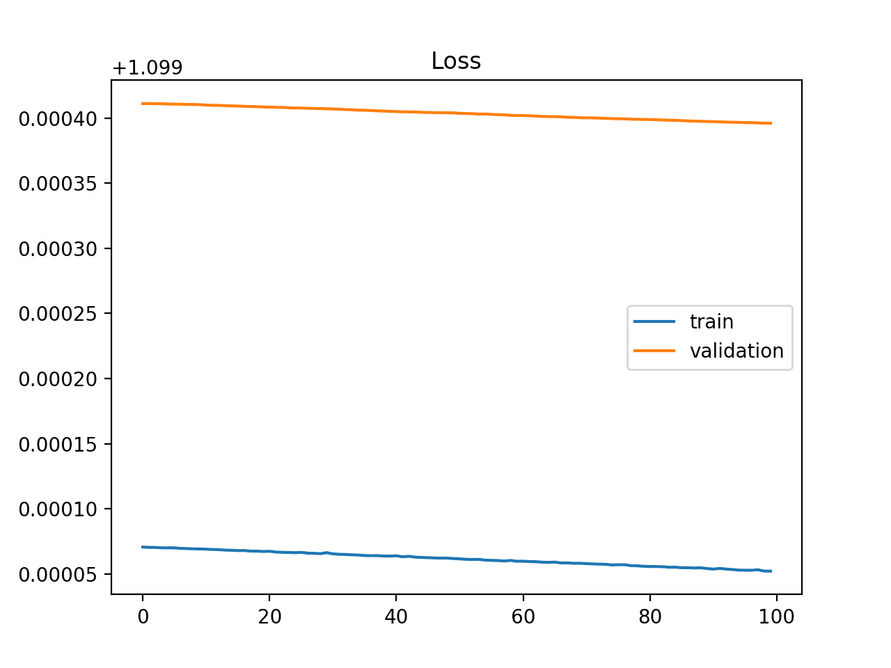
This would be your goal during training - a curve between an overfit and underfit model.

A good fit is usually identified be a training and validation loss that decrease to a point of stability with a minimal gap between the two final loss values.

The loss of the model will always be lower on the training dataset than the validation dataset. This means that we should expect some gap between the train and validation loss learning curves. This gap is referred to as the "generalization gap."

This example plot would show a well-fit model: