gadenbuie/nwss.md

## nwss.md

      
    Raw
  

              nwss.md
            
          
    library(tidyverse)
library(RSocrata)
library(glue)
library(gt)
The NWSS Public SARS-CoV-2 Wastewater Metric Data is sourced from
https://data.cdc.gov/Public-Health-Surveillance/NWSS-Public-SARS-CoV-2-Wastewater-Metric-Data/2ew6-ywp6.
if (!file.exists("nwss.csv")) {
  id <- "2ew6-ywp6"
  nwss <-
    glue("https://data.cdc.gov/resource/{id}.csv") |>
    read.socrata() |>
    as_tibble() |>
    write_csv("nwss.csv")

  download.file("https://data.cdc.gov/api/views/{id}.json", "nwss-metadata.json")
}
Read in the downloaded data and metadata. Fortunately, the metadata is
comprehensive and includes a full description of all of the columns in the
data set.
nwss <- readr::read_csv("nwss.csv")
#> Rows: 729698 Columns: 16
#> ── Column specification ────────────────────────────────────────────────────────
#> Delimiter: ","
#> chr  (7): wwtp_jurisdiction, reporting_jurisdiction, sample_location, key_pl...
#> dbl  (6): wwtp_id, sample_location_specify, population_served, ptc_15d, dete...
#> date (3): date_start, date_end, first_sample_date
#> 
#> ℹ Use `spec()` to retrieve the full column specification for this data.
#> ℹ Specify the column types or set `show_col_types = FALSE` to quiet this message.

meta <- jsonlite::fromJSON("nwss-metadata.json")
meta$columns |>
  as_tibble() |>
  select(name:description) |>
  gt() |>
  as_raw_html()

  
      name
      dataTypeName
      description
    
  
    wwtp_jurisdiction
text
State, DC, US territory, or Freely Associated State jurisdiction name (2-letter abbreviation) in which the wastewater treatment plant provided in 'wwtp_id' is located.
    wwtp_id
text
A unique identifier for wastewater treatment plants. This is an arbitrary integer used to provide a unique, but anonymous identifier for a wastewater treatment plant. This identifier is consistent over time, such that the same plant retains the same ID regardless of the addition or subtraction of other plants from the data set.
    reporting_jurisdiction
text
The CDC Epidemiology and Laboratory Capacity (ELC) jurisdiction, most frequently a state, reporting these data (2-letter abbreviation)
    sample_location
text
Sample collection location in the wastewater system, whether at a wastewater treatment plant (or other community level treatment infrastructure such as community-scale septic) or upstream in the wastewater system.
    sample_location_specify
text
A unique identifier for "upstream" sample locations. Specifically, when 'sample_location' is "upstream", this field has a non-empty value, which provides a unique, but anonymous identifier for the upstream sample collection sites. This identifier is consistent over time, such that the same sample collection site retains the same ID regardless of the addition or subtraction of other sample collection sites from the data set.
    key_plot_id
text
A unique identifier for the geographic area served by this sampling site, called a sewershed. This is an underscore-separated concatenation of the fields 'wwtp_jurisdiction', 'wwtp_id', and, if 'sample_location' is "upstream", then also 'sample_location_specify', and sample_matrix.
    county_names
text
The county and county-equivalent names corresponding to the FIPS codes in 'county_fips'
    county_fips
text
5-digit numeric FIPS codes of all counties and county equivalents served by this sampling site (i.e., served by this wastewater treatment plant or, if 'sample_location' is "upstream", then by this upstream location). Note that multiple sampling sites or treatment plants may serve a single county, and that a single sampling site or treatment plant may serve multiple counties. Counties listed may be entirely or only partly served by this sampling site.
    population_served
text
Estimated number of persons served by this sampling site (i.e., served by this wastewater treatment plant or, if 'sample_location' is "upstream", then by this upstream location).
    date_start
text
The start date of the interval over which the metric is calculated. Intervals are inclusive of start and end dates.
    date_end
text
The end date of the interval over which metric is calculated. Intervals are inclusive of start and end dates.
    ptc_15d
text
The percent change in SARS-CoV-2 RNA levels over the 15-day interval defined by 'date_start' and 'date_end'. Percent change is calculated as the modeled change over the interval, based on linear regression of log-transformed SARS-CoV-2 levels. SARS-CoV-2 RNA levels are wastewater concentrations that have been normalized for wastewater composition. 
    detect_prop_15d
text
The proportion of tests with SARS-CoV-2 detected, meaning a cycle threshold (Ct) value <40 for RT-qPCR or at least 3 positive droplets/partitions for RT-ddPCR, by sewershed over the 15-day window defined by 'date_start' and "date_end'. The detection proportion is the percent calculated by dividing the 15-day rolling sum of SARS-CoV-2 detections by the 15-day rolling sum of the number of tests for each sewershed and multiplying by 100.
    percentile
text
This metric shows whether SARS-CoV-2 virus levels at a site are currently higher or lower than past historical levels at the same site. 0% means levels are the lowest they have been at the site; 100% means levels are the highest they have been at the site. Public health officials watch for increasing levels of the virus in wastewater over time and use this data to help make public health decisions. 
    sampling_prior
text
Indicates whether the site was collecting wastewater samples before or on December 1, 2021.
    first_sample_date
text
The first date samples were collected at a site.
  
  
nwss |> glimpse()
#> Rows: 729,698
#> Columns: 16
#> $ wwtp_jurisdiction       <chr> "South Carolina", "South Carolina", "South Car…
#> $ wwtp_id                 <dbl> 2564, 2564, 2564, 2564, 2564, 2564, 2564, 2564…
#> $ reporting_jurisdiction  <chr> "South Carolina", "South Carolina", "South Car…
#> $ sample_location         <chr> "Treatment plant", "Treatment plant", "Treatme…
#> $ sample_location_specify <dbl> NA, NA, NA, NA, NA, NA, NA, NA, NA, NA, NA, NA…
#> $ key_plot_id             <chr> "CDC_VERILY_sc_2564_Treatment plant_post grit …
#> $ county_names            <chr> "Horry", "Horry", "Horry", "Horry", "Horry", "…
#> $ county_fips             <chr> "45051", "45051", "45051", "45051", "45051", "…
#> $ population_served       <dbl> 12000, 12000, 12000, 12000, 12000, 12000, 1200…
#> $ date_start              <date> 2023-12-19, 2023-12-20, 2023-12-21, 2023-12-2…
#> $ date_end                <date> 2024-01-02, 2024-01-03, 2024-01-04, 2024-01-0…
#> $ ptc_15d                 <dbl> NA, NA, -97, -97, -97, -97, -100, -100, -100, …
#> $ detect_prop_15d         <dbl> 100, 100, 100, 100, 100, 100, 100, 100, 100, 1…
#> $ percentile              <dbl> 79.000, 79.000, 75.000, 75.000, 75.000, 75.000…
#> $ sampling_prior          <chr> "no", "no", "no", "no", "no", "no", "no", "no"…
#> $ first_sample_date       <date> 2024-01-02, 2024-01-02, 2024-01-02, 2024-01-0…
My best (and quickest) guess is that the original plot posted by Dr. Lucky
Tran is something similar to or derived from the median
value of percentile by a date, either date_start, date_end or a
derivation of the two.

nwss |>
  summarize(value = median(percentile, na.rm = TRUE), .by = date_end) |>
  ggplot() +
  aes(date_end, value) +
  geom_line() +
  xlim(as.Date("2022-01-01"), as.Date("2024-04-15")) +
  ylim(0, 100)
#> Warning: Removed 545 rows containing missing values or values outside the scale range
#> (`geom_line()`).

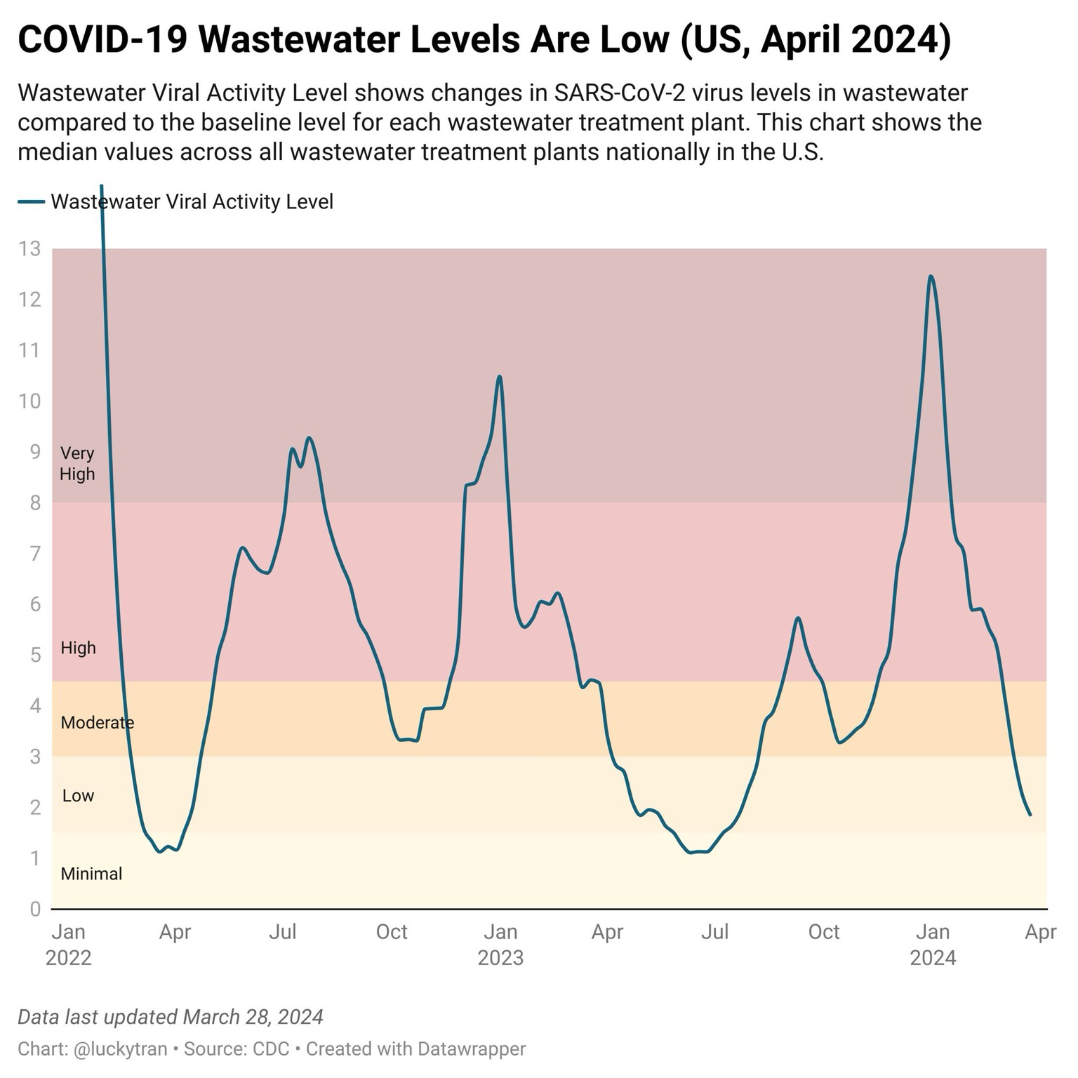
The CDC provides a summary of the “viral activity level” in a separate data
set at https://covid.cdc.gov/covid-data-tracker/#wastewater-surveillance.
Note that viral_activity_level is not provided in the original data set,
but it might be possible to derive its value from data in the original.
nwss_viral <- 
  read_csv(
    "wastewater_surveillance_viral_activity_level_over_time_data.csv",
    skip = 3,
    col_names = c("date", "viral_activity_level"),
    col_types = cols(
      date = col_date(),
      viral_activity_level = col_double()
    )
  )
  
nwss_viral |>
  rowwise() |>
  mutate(viral_activity_level = min(viral_activity_level, 13)) |>
  ggplot() +
  aes(date, viral_activity_level) + 
  geom_line() +
  scale_y_continuous(breaks = 0:13, expand = c(0, 0), limits = c(0, 13))

Under Data Methods in About Wastewater Data this paragraph describes how viral activity levels are calculated (emphasis original):

About the Wastewater Viral Activity Level: The Wastewater Viral Activity Level is a calculated measure that allows us to aggregate wastewater sample data to get state/territorial, regional, and national levels and see trends over time. Most simply, the value associated with the Wastewater Viral Activity Level is the number of standard deviations above the baseline, transformed to the linear scale. The current Wastewater Viral Activity Level for each state and territory is categorized into minimal, low, moderate, high, or very high as follows: a Wastewater Viral Activity Level less than 1.5 is categorized as minimal, greater than 1.5 and up to 3 is low, greater than 3 and up to 4.5 is moderate, greater than 4.5 and up to 8 is high, and greater than 8 is very high.
name	dataTypeName	description
wwtp_jurisdiction	text	State, DC, US territory, or Freely Associated State jurisdiction name (2-letter abbreviation) in which the wastewater treatment plant provided in 'wwtp_id' is located.
wwtp_id	text	A unique identifier for wastewater treatment plants. This is an arbitrary integer used to provide a unique, but anonymous identifier for a wastewater treatment plant. This identifier is consistent over time, such that the same plant retains the same ID regardless of the addition or subtraction of other plants from the data set.
reporting_jurisdiction	text	The CDC Epidemiology and Laboratory Capacity (ELC) jurisdiction, most frequently a state, reporting these data (2-letter abbreviation)
sample_location	text	Sample collection location in the wastewater system, whether at a wastewater treatment plant (or other community level treatment infrastructure such as community-scale septic) or upstream in the wastewater system.
sample_location_specify	text	A unique identifier for "upstream" sample locations. Specifically, when 'sample_location' is "upstream", this field has a non-empty value, which provides a unique, but anonymous identifier for the upstream sample collection sites. This identifier is consistent over time, such that the same sample collection site retains the same ID regardless of the addition or subtraction of other sample collection sites from the data set.
key_plot_id	text	A unique identifier for the geographic area served by this sampling site, called a sewershed. This is an underscore-separated concatenation of the fields 'wwtp_jurisdiction', 'wwtp_id', and, if 'sample_location' is "upstream", then also 'sample_location_specify', and sample_matrix.
county_names	text	The county and county-equivalent names corresponding to the FIPS codes in 'county_fips'
county_fips	text	5-digit numeric FIPS codes of all counties and county equivalents served by this sampling site (i.e., served by this wastewater treatment plant or, if 'sample_location' is "upstream", then by this upstream location). Note that multiple sampling sites or treatment plants may serve a single county, and that a single sampling site or treatment plant may serve multiple counties. Counties listed may be entirely or only partly served by this sampling site.
population_served	text	Estimated number of persons served by this sampling site (i.e., served by this wastewater treatment plant or, if 'sample_location' is "upstream", then by this upstream location).
date_start	text	The start date of the interval over which the metric is calculated. Intervals are inclusive of start and end dates.
date_end	text	The end date of the interval over which metric is calculated. Intervals are inclusive of start and end dates.
ptc_15d	text	The percent change in SARS-CoV-2 RNA levels over the 15-day interval defined by 'date_start' and 'date_end'. Percent change is calculated as the modeled change over the interval, based on linear regression of log-transformed SARS-CoV-2 levels. SARS-CoV-2 RNA levels are wastewater concentrations that have been normalized for wastewater composition.
detect_prop_15d	text	The proportion of tests with SARS-CoV-2 detected, meaning a cycle threshold (Ct) value <40 for RT-qPCR or at least 3 positive droplets/partitions for RT-ddPCR, by sewershed over the 15-day window defined by 'date_start' and "date_end'. The detection proportion is the percent calculated by dividing the 15-day rolling sum of SARS-CoV-2 detections by the 15-day rolling sum of the number of tests for each sewershed and multiplying by 100.
percentile	text	This metric shows whether SARS-CoV-2 virus levels at a site are currently higher or lower than past historical levels at the same site. 0% means levels are the lowest they have been at the site; 100% means levels are the highest they have been at the site. Public health officials watch for increasing levels of the virus in wastewater over time and use this data to help make public health decisions.
sampling_prior	text	Indicates whether the site was collecting wastewater samples before or on December 1, 2021.
first_sample_date	text	The first date samples were collected at a site.