Skip to content

Instantly share code, notes, and snippets.

@hrbrmstr
Last active June 30, 2019 12:09
Show Gist options
  • Star 16 You must be signed in to star a gist
  • Fork 3 You must be signed in to fork a gist
  • Save hrbrmstr/0d206070cea01bcb0118 to your computer and use it in GitHub Desktop.
Save hrbrmstr/0d206070cea01bcb0118 to your computer and use it in GitHub Desktop.

This hit #rstats today:

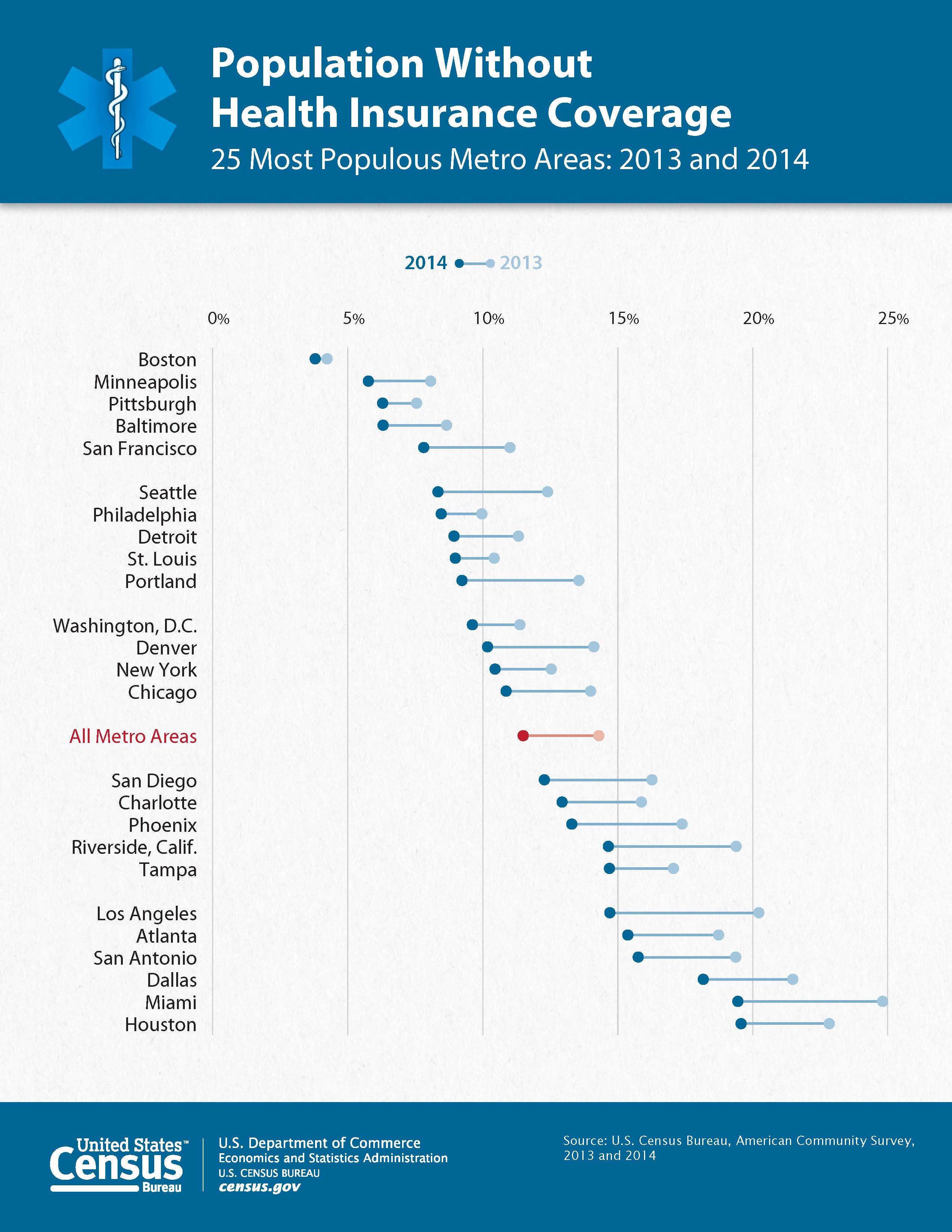
Has anyone made a dumbbell dot plot in #rstats, or better yet exported to @plotlygraphs using the API? https://t.co/rWUSpH1rRl

— Ken Davis (@ken_mke) October 23, 2015
<script async src="//platform.twitter.com/widgets.js" charset="utf-8"></script>

So, I figured it was worth a cpl mins to reproduce.

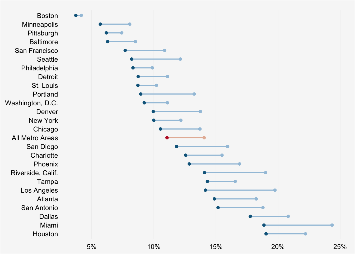
While the US gov did give the data behind the chart it was all the data and a pain to work with so I used WebPlotDigitizer to transcribe the points and then some data wrangling in R to clean it up and make it work well with ggplot2.

It is possible to make the top "dumbbell" legend in ggplot2 (but not by using a guide) and color the "All Metro Areas" text but that's an exercise left to the reader (totally doable and not much code, but not the point of the example).

library(dplyr)
library(tidyr)
library(scales)
library(ggplot2)
library(ggalt) # devtools::install_github("hrbrmstr/ggalt")
health <- read.csv("zhealth.csv", stringsAsFactors=FALSE,
header=FALSE, col.names=c("pct", "area_id"))
areas <- read.csv("zarea_trans.csv", stringsAsFactors=FALSE, header=TRUE)
health %>%
mutate(area_id=trunc(area_id)) %>%
arrange(area_id, pct) %>%
mutate(year=rep(c("2014", "2013"), 26),
pct=pct/100) %>%
left_join(areas, "area_id") %>%
mutate(area_name=factor(area_name, levels=unique(area_name))) -> health
setNames(bind_cols(filter(health, year==2014), filter(health, year==2013))[,c(4,1,5)],
c("area_name", "pct_2014", "pct_2013")) -> health
gg <- ggplot(health, aes(x=pct_2013, xend=pct_2014, y=area_name, group=area_name))
gg <- gg + geom_dumbbell(color="#a3c4dc", size=0.75, point.colour.l="#0e668b")
gg <- gg + scale_x_continuous(label=percent)
gg <- gg + labs(x=NULL, y=NULL)
gg <- gg + theme_bw()
gg <- gg + theme(plot.background=element_rect(fill="#f7f7f7"))
gg <- gg + theme(panel.background=element_rect(fill="#f7f7f7"))
gg <- gg + theme(panel.grid.minor=element_blank())
gg <- gg + theme(panel.grid.major.y=element_blank())
gg <- gg + theme(panel.grid.major.x=element_line())
gg <- gg + theme(axis.ticks=element_blank())
gg <- gg + theme(legend.position="top")
gg <- gg + theme(panel.border=element_blank())
gg
library(dplyr)
library(ggplot2)
library(scales)
health <- read.csv("zhealth.csv", stringsAsFactors=FALSE,
header=FALSE, col.names=c("pct", "area_id"))
areas <- read.csv("zarea_trans.csv", stringsAsFactors=FALSE, header=TRUE)
health %>%
mutate(area_id=trunc(area_id)) %>%
arrange(area_id, pct) %>%
mutate(year=rep(c("2014", "2013"), 26),
pct=pct/100) %>%
left_join(areas, "area_id") %>%
mutate(area_name=factor(area_name, levels=unique(area_name))) %>%
mutate(color=rep(c("#0e668b", "#a3c4dc"), 26),
line_col="#a3c4dc") -> health
health[health$area_name=="All Metro Areas",]$color <- c("#bc1f31", "#e5b9a5")
health[health$area_name=="All Metro Areas",]$line_col <- "#e5b9a5"
gg <- ggplot(health)
gg <- gg + geom_path(aes(x=pct, y=area_name, group=area_id, color=line_col), size=0.75)
gg <- gg + geom_point(aes(x=pct, y=area_name, color=color), size=2.25)
gg <- gg + scale_color_identity()
gg <- gg + scale_x_continuous(label=percent)
gg <- gg + labs(x=NULL, y=NULL)
gg <- gg + theme_bw()
gg <- gg + theme(plot.background=element_rect(fill="#f7f7f7"))
gg <- gg + theme(panel.background=element_rect(fill="#f7f7f7"))
gg <- gg + theme(panel.grid.minor=element_blank())
gg <- gg + theme(panel.grid.major.y=element_blank())
gg <- gg + theme(panel.grid.major.x=element_line())
gg <- gg + theme(axis.ticks=element_blank())
gg <- gg + theme(legend.position="top")
gg <- gg + theme(panel.border=element_blank())
gg
area_id area_name
0 Houston
1 Miami
2 Dallas
3 San Antonio
4 Atlanta
5 Los Angeles
7 Tampa
8 Riverside, Calif.
9 Phoenix
10 Charlotte
11 San Diego
13 All Metro Areas
15 Chicago
16 New York
17 Denver
18 Washington, D.C.
20 Portland
21 St. Louis
22 Detroit
23 Philadelphia
24 Seattle
26 San Francisco
27 Baltimore
28 Pittsburgh
29 Minneapolis
30 Boston
22.209907307969008 0.19674900165782105
19.036743162789726 0.25618033761169556
18.86689466056366 1.159849440615588
24.347402225025796 1.3381434484772043
17.766163759396925 2.2095945114639974
20.81765006412328 2.3003054979199007
15.171516750252842 3.251832466191914
18.783221595470707 3.3453586211930073
14.875767654756068 4.079492018475847
18.24130165052289 4.32253490287669
19.752108769771347 5.234649511516132
14.151330949128862 5.281881783774203
16.551887726907797 7.1783669937127925
14.312421149214359 7.24249027724197
14.080326142489234 8.145846583740841
18.99920758218728 8.245941465347371
12.856509816596983 9.270350019289118
16.902532609035646 9.290681792115443
12.563575889645392 10.248777486992886
15.489161601101042 10.263478922728844
11.834916431200408 11.225015379161505
15.943185728138129 11.24565994849285
14.050141279754765 13.195946157294934
11.06371664807265 13.256315882763872
10.537280130123342 15.06271569925659
13.71325944384781 15.154052278722538
9.998175353720711 16.190659896360096
12.176803011187687 16.20160777403581
13.75126421920779 17.189419136890177
9.955635029037943 17.245722507793847
9.226975570592955 18.221960399962466
11.095778289837238 18.30672825282299
8.950932654912467 20.104995360185175
13.247349049619952 20.201962276741494
8.721652816732526 21.159119582103873
10.215568924709881 21.166626698224363
11.105318583240361 22.15099729952351
8.741358996548808 22.21449499004265
8.323932060599105 23.192296864736363
9.880094673075519 23.200116777361874
8.216330062872094 24.096278764245277
12.13785984631265 24.11598494406156
7.694116297740564 26.12883045386773
10.86868802719244 26.14478307562377
8.52161945177199 27.112888258661858
6.2821528740785535 27.177011542191035
6.175958460624134 28.15637739940986
7.420888550605261 28.162633329510268
5.693469851630191 29.983098562178736
8.061652191139517 29.14575274478933
3.725510640294443 30.254616355086593
4.16123617178784 30.256805930621738
Sign up for free to join this conversation on GitHub. Already have an account? Sign in to comment