The following repository helps you learn how to create a dataset from end-to-end and performing some data exploration and vizualization.
To implement data visualization in R programming, you should have some interest for data you use daily either in your job or at uni. Before I created this gist, I imagined how my data visualization could be of interest to Hadoop professionals on social networks since ultimately I share my gist to my Twitter and Linkedin followers. I therefore decided to find some available data related to this technology that could be interesting, to create a dataset in which I would use these data, to read this dataset using R, to perfom some analysis and cleaning operations on this dataset and to create a vizualisation chart that could tell a story about this dataset.
The following steps will help you visualize "the number of nodes in a Hadoop cluster used by major tech companies" (the story that I want to tell). To implement what I did, you may wish to proceed as follows:
- you can follow the below steps to understand all the steps from end-to-end
- or you can use program.rda in R Studio or in your favorite workbench to check the output
Steps
- Check https://who.is for retrieving data you'll use in your dataset (e.g: search for https://last.fm)
- Open your favorite text editor
- Name your columns company, nodes, country, server_type, server_version, Id
- Create 20 observations (an observation is equal to a row, 20 obs = 20 rows)
- Make sure to store data in each cell of your dataset (if you have no available data, use "NA"
- Save your file in
.csv - Make sure you have
RStudioinstalled on your machine (see Running the tests) - Open your file with R and vizualize it
- Create a new
Rscript, install and load the packages (refer to Tips.md - Open your
.csvin R and explore the data (refer to Tips.md to know how
I am using Ubuntu (18.04 bionic).
- Check on your shell if R Studio is correctly installed using this:
Check RStudio version
$ R --versionCheck Jupyter Notebook version
$ jupyter --versionYou need RStudio and Jupyter Nptebook installed on your PC to proprely use this gist.
Jupyter Notebook is not compulsory. It is another way to read R programming scripts.
You can still use Jupyter Notebook on remote sites to perform same operations you would perform in RStudio.
- use https://labs.cognitiveclass.ai (create a free account, then click on "JupyterLab" in the Build Analytics section)
- use https://dataplatform.ibm.com (recommended for IBM Coders)
- Notepadqq - A text editor - Linux/Unix
- R Studio - A statistical computing environment
- ggvis - a package for creating histograms
- ggplot2 - a famous package for plotting in
R
- This dataset was created using notepadqq.
- Data is sorted by company name, number of nodes, country name, server type, server version and position in the table.
- Save the code below in .csv and read it using RStudio before you invoke vizualisation functions.
- Data are provided by various sites. Some of them are listed in Tips.md
I used no vesioning system for this gist. My repository's status is flagged as active because it has reached a stable, usable state. Original gist related to this repository is pending as concept.
- Isaac Arnault
All public gists https://gist.github.com/isaacarnault
Copyright 2018, Isaac Arnault
MIT License, http://www.opensource.org/licenses/mit-license.php
As an IT or Big Data Project Manager, your are asked by the Information System Manager to use a dataset in order to do some presentation regarding the management of Hadoop clusters all over the world. For your presentation, you have decided to include some metrics related to the number of nodes processed by top Internet companies and to locate the servers on which the nodes are processed by Internet Protocol address. Since some data are available in the Public Domain (on the Internet), you have decided to go for them. This excercise is only a part of a whole set of steps you'd have conducted on top of your presentation (Business understanding, Analytic approach, Data requirements / - collection / - analysis / - preparation, - modeling). Completing this exercise could be seen as a prerequisite regarding data analysis for enterprise.
- Create your dataset by using data from this Slideshare
- Consider the following range of data while extracting them from the above link: dataset = {2, 21}
- Name the variables of your dataset Id, Company, Nodes, Country, Server
- Go to Tips.md to find sources where you can find Server name and Country
- Assign to each Id a Company, number of Nodes, Country and Server Name
- Read your dataset using
RStudioorJupyter - Use
Jupyterto perform some exploration of your dataset - Use
RStudioto perform some visualisation of your dataset:- Install and activate ggvis and ggplot2 packages from the CRAN
- Use geom_dotplot function for plotting. Sort the graph by Company per Nodes.
- Question: How many companies use {500, 1500} nodes? Name the companies while visualizing the graph.