Illustrates Lorentz contraction of an accelerating rocket. (special relativity)

LorentzContractionOfAccelRocket.tex

\documentclass[crop=true, border=10pt]{standalone}
\usepackage{comment}
\begin{comment} 
:Title: Lorentz contraction of an accelerated rocket
:Slug: Lorentz contraction
:Tags:  special relativity
:Author: J A Miller, UAH Physics & Astronomy, millerja@uah.edu, 2020/05/28

Illustration of length contraction during acceleration.

Basic plot style and colors from:
    https://gist.github.com/mcnees/45b9f53ad371c38ba6f3759df5880fb1

---------------------------------------------------------------------
Background
---------------------------------------------------------------------

Recall: The equations of motion for a point object undergoing uniform proper acceleration $\alpha$ are
\begin{equation}
    \begin{split}
		x &= \frac{1}{\alpha} \cosh(\alpha \tau) - \frac{1}{\alpha} + x_0 \\
		t &= \frac{1}{\alpha} \sinh(\alpha \tau),
    \end{split}
\end{equation}
where $\tau$ is the proper time, and $x_0$ is the starting location.

A question is whether Lorentz contraction of a finite-length object (e.g., a rocket) occurs as expected. This can be a very tricky question to answer, since you just cannot take a slice in the $x$ direction at some $t$ and find the distance between the worldline, like we have always done before. The reason you can't is because those two points are moving with different speeds in the lab frame, and so there is not a common rest frame.

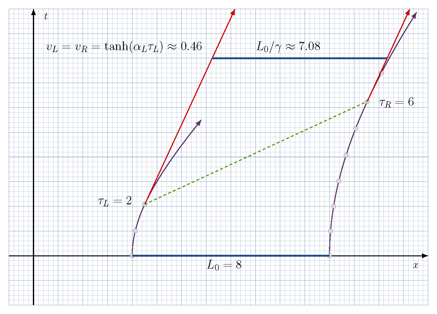
We will approach the problem thusly. Suppose, for example, in the previous figure we consider the left proper time $\tau_L$. This is simultaneous with the right proper time $\tau_R = \tau_L \alpha_L/\alpha_R$, and at those times the ends have the same velocity $v_L = v_R$. This is one thing we need. We show this in Figure for $\tau_L = 2$ for illustration. 

Now suppose that proper acceleration stops in the rocket frame. All points on the rocket then coast with constant velocity $v_L$, and the ends will have straight worldlines like our previous examples. We can let Mathematica do some work here and find the equations for the straight lines (e.g., they will have the same slope $1/v_L = 1/v_R$, where $v_L = \tanh(\xlpha_L \tau_L)$). Then it is a simple matter to find the distance between them at any lab time $t$, which turns out to be
\begin{equation}
	\begin{split}
		x_R - x_L &= L_0 \sech(\alpha_L \tau_L) \\
		                &= \frac{L_0}{\gamma(\tau)},
	\end{split}
\end{equation}
since, again, $v_L = \tanh(\alpha_L \tau_L)$. (If needed for some reason, it's easy to convert from proper to lab time in $\gamma$.) Hence, Lorentz contraction occurs as required.

Figure caption:
\caption{Same as Fig. \ref{fig-rocket}, but showing only a portion of the left and right rocket ends. \textit{Red arrows:} Worldlines after proper acceleration ceases along the rocket. \texit{Heavy blue line:} The star frame rocket length.} 

\end{comment}



\usepackage{tikz}
\usetikzlibrary{arrows.meta}

\usepackage{pgfplots}
\pgfplotsset{compat=1.16}

\usepackage{xcolor}
\definecolor{plum}{rgb}{0.36078, 0.20784, 0.4}
\definecolor{chameleon}{rgb}{0.30588, 0.60392, 0.023529}
\definecolor{cornflower}{rgb}{0.12549, 0.29020, 0.52941}
\definecolor{scarlet}{rgb}{0.8, 0, 0}
\definecolor{brick}{rgb}{0.64314, 0, 0}
\definecolor{sunrise}{rgb}{0.80784, 0.36078, 0}
\definecolor{lightblue}{rgb}{0.15,0.35,0.75}


% ----------------------- user specifications ------------------------

% Note: these really aren't free. The calcuations of the worldlines after acceleration
% is removed is a chore. This is done one for the parameters listed here. If you change, them
% have some fixing to do in drawing the acceleration-free worldlines.

% proper acceleration of the left end
\newcommand*{\accelL}{0.25}

% starting point of left end
\pgfmathsetmacro{\xinitL}{1/\accelL}

% maximum proper time for the left end
\newcommand*{\taumaxL}{2.5}

% proper length of rocket
\newcommand*{\length}{8}  

% ---------------------- calculations and functions -------------------

% proper acceleration of the right end
\pgfmathsetmacro{\accelR}{\accelL/(1+\accelL*\length}

% maximum proper time for the right end
\pgfmathsetmacro{\taumaxR}{\taumaxL*\accelL/\accelR}

% define left worldline as a function of its proper time
\pgfkeys{/pgf/declare function={xL(\tau) = (1/\accelL)*(cosh(\accelL*\tau)-1)+\xinitL;}}
\pgfkeys{/pgf/declare function={tL(\tau) = (1/\accelL)*sinh(\accelL*\tau);}}

% define right worldline as a function of its proper time
\pgfkeys{/pgf/declare function={xR(\tau) = (1/\accelR)*(cosh(\accelR*\tau)-1)+\xinitL+\length;}}
\pgfkeys{/pgf/declare function={tR(\tau) = (1/\accelR)*sinh(\accelR*\tau);}}

 
 
% ---------------------- figure ------------------------------------------

% Set the point style for the proper time ticks
\tikzset{
	taudot/.style={circle,draw=plum!70,fill=plum!20,inner sep=1.75pt} 
 }

\begin{document}


\begin{tikzpicture}[scale=1,domain=-1:16]
	\tikzstyle{axisarrow} = [-{Latex[inset=0pt,length=7pt]}]


	% Draw the background grid.
	\draw [cornflower!30,step=0.2,thin] (-1,-2) grid (16,10);
	\draw [cornflower!60,step=1.0,thin] (-1,-2) grid (16,10);

	% Clip everything that falls outside the grid
	\clip(-1,-2) rectangle (16,10);
	
	% Draw Axes
	\draw[thick,axisarrow] (0,-2) -- (0,10);
	\node[inner sep=0pt] at (0.5,9.7) {\large $t$};
	\draw[thick,axisarrow] (-1,0) -- (16,0);
	\node[inner sep=0pt] at (15.5,-0.4) {\large $x$};

	% Left end of rocket
	\draw[domain=0:\taumaxL+2,smooth,variable=\tauL,plum,thick,axisarrow] plot ({xL(\tauL)},{tL(\tauL)});

	% Mark units one proper time interval apart
    \foreach \tauL in {0,1,2,...,\taumaxL}
	{
			\node[taudot]  at ({xL(\tauL)},{tL(\tauL)}) {};
	}	
	
	% Right end of rocket. Don't forget to scale the proper time
	\draw[domain=0:\taumaxR+1.5,smooth,variable=\tauR,plum,thick,axisarrow] plot ({xR(\tauR)},{tR(\tauR)});

	% Mark units one proper time interval apart
    \foreach \tauR in {0,1,2,...,\taumaxR}
	{
			\node[taudot]  at ({xR(\tauR},{tR(\tauR)}) {};
	}	

	% Here is where we draw the motion after the acceleration ends. The calculations
	% are cumbersome in tikz, so we just the parameters given above
	\draw[thick,axisarrow,scarlet] ({xL(2)},{tL(2)}) -- (8.17,10);
	\draw[thick,axisarrow,scarlet] ({xR(6)},{tR(6)}) -- (15.26,10);
	
	% draw line of simultaneity and simultaneous velocity
	\draw[thick,chameleon,dashed] ({xL(2)},{tL(2)}) --({xR(6)},{tR(6)}) ;
	
	% draw the rocket
	% Draw train length in unprimed frame
  \draw[line width=2,cornflower] (\xinitL,0) -- (\xinitL+\length,0);
  \draw[line width=2,cornflower] (7.244,8) -- (14.33,8);	
    
  % Some more labels	
  \node[above left,inner sep=0pt] at (4,2) {\Large $\tau_L = 2$};
  \node[above right,inner sep=0pt] at (14,6) {\Large $\tau_R = 6$};
	\node[above right,inner sep=0pt] at (0.5,8.2) {\Large $v_L = v_R = \tanh(\alpha_L \tau_L) \approx 0.46$};
	\node[above right,inner sep=0pt] at (9,8.2) {\Large $L_0/\gamma \approx 7.08$};
	\node[above right,inner sep=0pt] at (7,-0.6) {\Large $L_0 =  8$};
	
	
	
\end{tikzpicture}
			

\end{document}

Figure from above code.