Skip to content

Instantly share code, notes, and snippets.

@jessstringham
Last active November 17, 2017 09:46
Show Gist options
  • Star 0 You must be signed in to star a gist
  • Fork 0 You must be signed in to fork a gist
  • Save jessstringham/827d8582eb4e3e0c26e9b16f6105621a to your computer and use it in GitHub Desktop.
Save jessstringham/827d8582eb4e3e0c26e9b16f6105621a to your computer and use it in GitHub Desktop.
Bayesian linear regression with polynomial basis functions

Srry, this is a bit of an awkward format. I might move this and a few other demos to a repo.

This is code one could drop into Jupyter [1] notebook cells and draw some wicked-looking graphs. I wrote it to understand Bayesian linear regression (for this classMLPR, specifically this and this). No promises that I did it perfectly.

The graphs show samples from the posterior weights in pink. The black lines kinda show the posterior distribution P(y|data) by drawing lines for standard deviations away from the mean. So it goes through the points on the x-axis, asks P(y|data) for the value and uncertainty

It uses polynomial basis functions, because they are sqiggly and cool-looking.

  • model_params=3 matches the underlying function (and the right noise variance sigma_y is already set)
  • If you set "sample size" to 0, you can see the prior. Then try messing with sigma_w. This demo uses the same sigma_w for all weights. You can also see the impact of the prior after data.
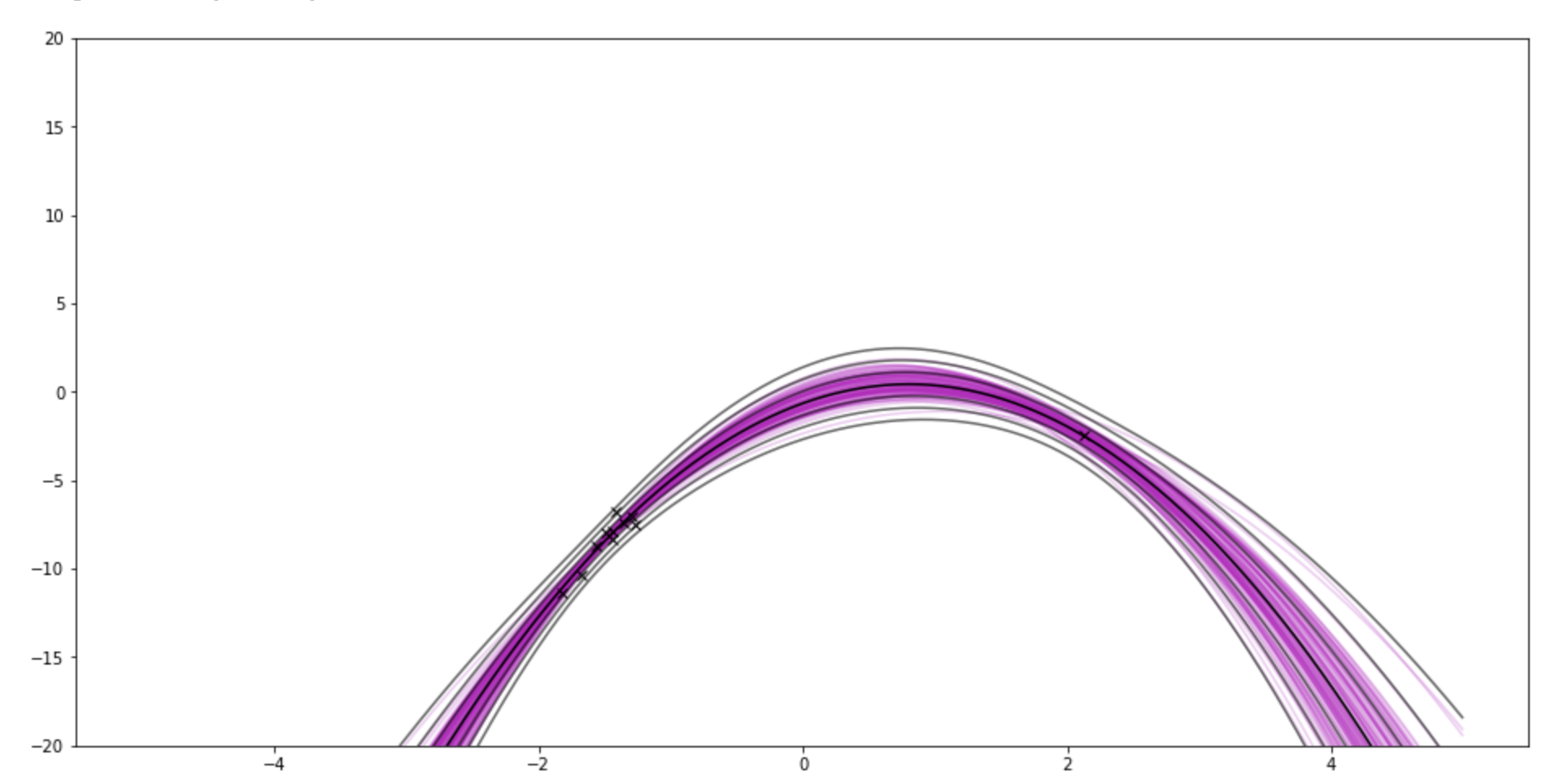
  • For fun, I sample from two regions of the underlying function. So try going from sample_size 10 to 11.
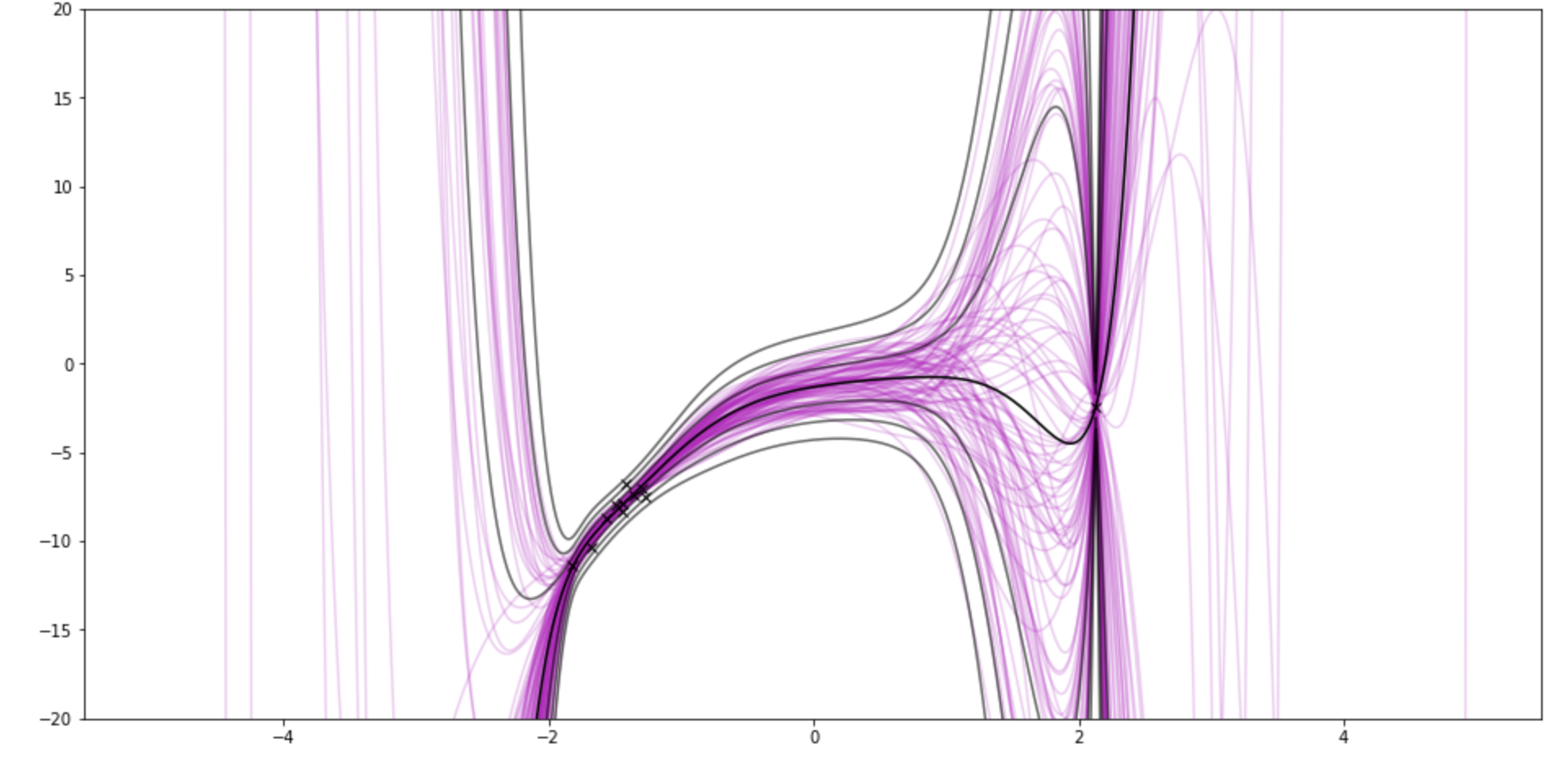
    • If you set the "model–params" (number of coefficients) to 10 and sample size to 11, it pinches around the brand new point.

[1] with matplotlib, numpy, scipy

import matplotlib.pyplot as plt
import numpy as np
from ipywidgets import interact, interact_manual
from scipy.linalg import cholesky
from scipy.stats import multivariate_normal
# weights for the underlying function
real_w = np.vstack((0.5, 3, -2))
def generate_noisy_samples(sample_size, actual_sigma_y, real_w):
# sample sample_size points between -2, 2
#X_in = np.random.rand(sample_size, 1) * 4 - 2
# sample approx sample_size points near -2 and 2
X_in = np.vstack((
np.random.rand(int(sample_size / 2), 1) - 2,
np.random.rand(int(sample_size / 2), 1) + 2
))
f = np.hstack(X_in**i for i in range(len(real_w))) @ real_w
noise = actual_sigma_y * np.random.randn(X_in.shape[0], 1)
y = f + noise
assert y.shape == (sample_size, 1)
return X_in, y
all_X_in, all_y = generate_noisy_samples(
sample_size=20,
actual_sigma_y=.4,
real_w=real_w,
)
N = 100 # number of lines
grid_size = 0.01
x_grid = np.arange(-5, 5, grid_size)
def plot_example(model_params, sample_size, sigma_w):
# For fun graphics, we use the first `sample_size` points.
X_in = all_X_in[:sample_size]
y = all_y[:sample_size]
# Set our guesses of sigma
#sigma_w = 1 # weights
sigma_y = .4 # noisy observations
# Set up the prior
w_0 = np.tile(0, (model_params, 1))
V_0 = sigma_w**2 * np.identity(model_params)
# Compute phi for our X_in
Phi_X_in = np.hstack(X_in**i for i in range(model_params))
# Now compute the posterior, just reading off the formula
V0_inv = np.linalg.inv(V_0)
V_n = sigma_y**2 * np.linalg.inv(sigma_y**2 * V0_inv + (Phi_X_in.T @ Phi_X_in))
w_n = V_n @ V0_inv @ w_0 + 1 / (sigma_y**2) * V_n @ Phi_X_in.T @ y
assert w_n.shape == (model_params, 1)
# Now let's draw!
# Now we're ready to start plotting.
# This is the X for the entire grid
X = np.vstack(x_grid**i for i in range(model_params)).T
plt.clf()
plt.figure(figsize=(16, 8))
# here are some posterior lines
w = np.random.multivariate_normal(mean=w_n.flatten(), cov=V_n, size=N)
plt.plot(x_grid, X @ w.T, '-m', alpha=.2)
# here's the mean
plt.plot(x_grid, X @ w_n, '-w')
# How curvey can this be?
var_post = np.sum(np.dot(X, V_n) * X, 1)[:, None] + sigma_y**2
for k in np.arange(1, 4):
plt.plot(x_grid, X @ w_n + k * np.sqrt(var_post), '-', color='0.2')
plt.plot(x_grid, X @ w_n - k * np.sqrt(var_post), '-', color='0.2')
# here is the prior
#plt.plot(x_grid, X @ w_0, '-g')
# here's f
#plt.plot(x_grid, np.vstack([x_grid**i for i in range(len(real_w))]).T @ real_w, '-b')
# here is samples
plt.plot(X_in, y, 'xk')
# here are the points used in the posterior
plt.ylim([-20, 20])
plt.show()
interact(
plot_example,
model_params=(1, 10),
sample_size=(0, 20),
sigma_w=(0.1, 3),
continuous_update=False,
)
@jessstringham
Copy link
Author

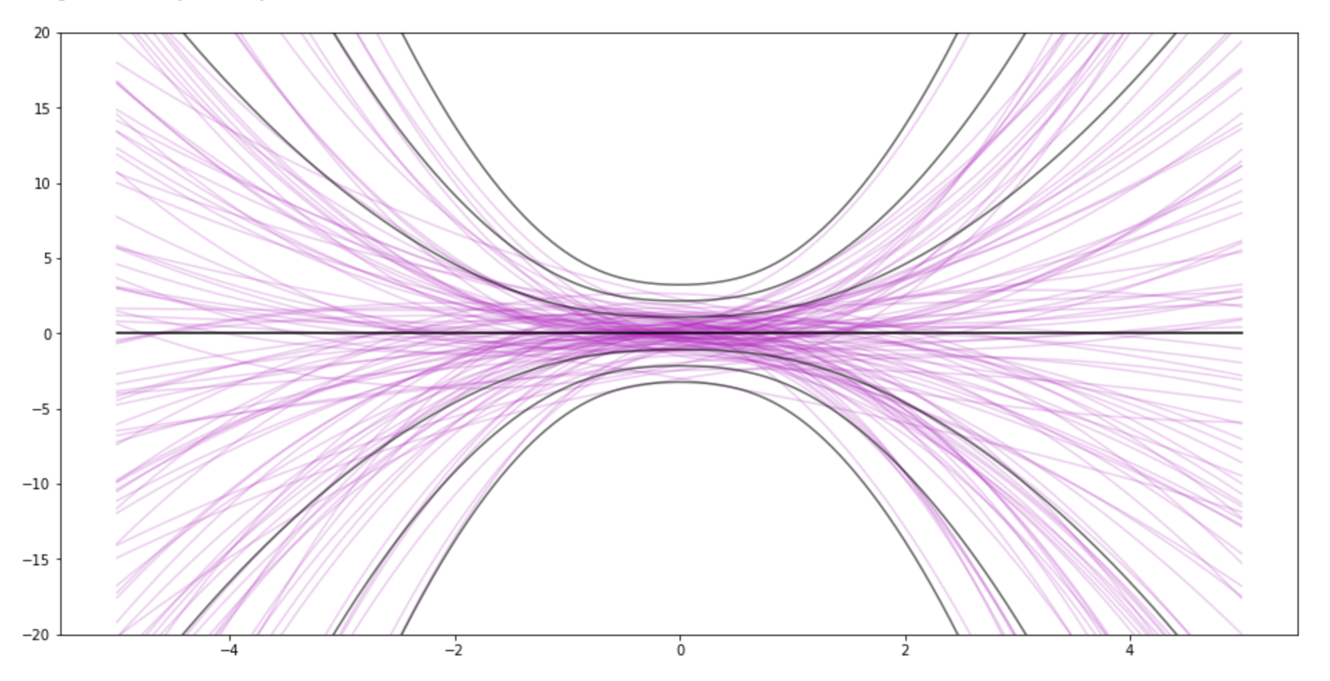
This is the prior for 3 weights (quadratic)
screen shot 2017-11-17 at 9 41 48 am

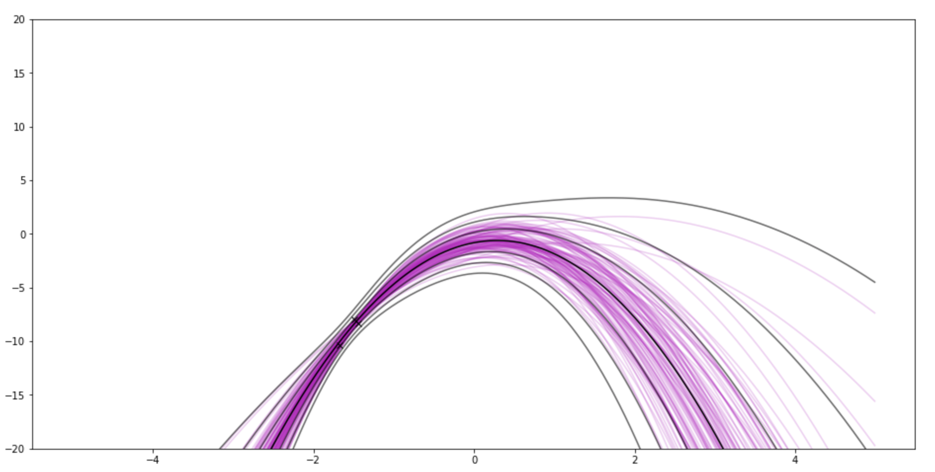
After 3 observations. There's still a little lump around 0.
screen shot 2017-11-17 at 9 42 05 am

After 11:
screen shot 2017-11-17 at 9 45 33 am

If I use 9-degree polynomial, and show 11 samples (10 from one side, 1 from another side)
screen shot 2017-11-17 at 9 43 08 am

Sign up for free to join this conversation on GitHub. Already have an account? Sign in to comment