coal_latent.R

# See page 209 of Stan reference manual
# https://pymc-devs.github.io/pymc/tutorial.html?highlight=change%20point

library(rstan)
library(boot)
library(dplyr)

# ---- Prep data ----
data(coal)
coal$year <- floor(coal$date)
coal_tab <- data.frame(table(coal$year), stringsAsFactors = FALSE)
names(coal_tab) <- c("year", "rate")
coal_tab$year <- as.numeric(as.character(coal_tab$year))

year_seq <- seq(from = range(as.numeric(as.character(coal_tab$year)))[1], 
                to   = range(as.numeric(as.character(coal_tab$year)))[2], 
                by = 1)

coal_missing <- data.frame(
  year = year_seq[
    !(year_seq %in% as.numeric(as.character(coal_tab$year)))], 
  rate = 0)

coal_tab <- rbind(coal_tab, coal_missing)
coal_tab <- coal_tab[order(coal_tab$year),]

# ---- Fit model ----
dataList <- list(T = nrow(coal_tab), D = coal_tab$rate, r_l = 1, r_e = 1)
stan_mod <- stan_model(file = "coal_latent.stan")
fit      <- sampling(stan_mod, dataList)

# ---- Create plots ----
year_index <- data.frame(year = coal_tab$year, index = seq_len(nrow(coal_tab)))
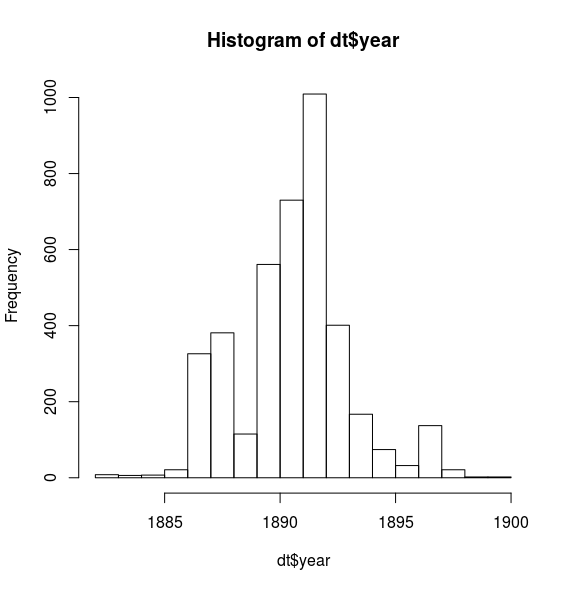
dt         <- data.frame(extract(fit, pars = "s"))
names(dt)  <- "index"
dt         <- left_join(dt, year_index)
hist(dt$year)

coal_latent.stan

// Dt:     Number of disasters in year t.
// rt:     Rate parameter of the Poisson distribution of disasters in year t.
// s:      Year in which the rate parameter changes (the switchpoint).
// e:      Rate parameter before the switchpoint s.
// l:      Rate parameter after the switchpoint s.
// tl, th: Lower and upper boundaries of year t.
// re, rl: Rate parameters of the priors of the early and late rates.

data {
  real<lower=0>r_l;
  real<lower=0>r_e;
  int<lower=1> T;
  int<lower=0> D[T];
}

transformed data {
  real log_unif;
  log_unif = -log(T);
}

parameters {
  real<lower=0> e;
  real<lower=0> l;
}

transformed parameters {
  vector[T] lp;
  lp = rep_vector(log_unif, T);
  for (s in 1:T)
    for (t in 1:T)
      lp[s] = lp[s] + poisson_lpmf(D[t] | t < s ? e : l);
}

model {
  e ~ exponential(r_e);
  l ~ exponential(r_l);
  target += log_sum_exp(lp);
}

generated quantities {
  int<lower=1,upper=T> s;
  s = categorical_logit_rng(lp);
}