You signed in with another tab or window. Reload to refresh your session.You signed out in another tab or window. Reload to refresh your session.You switched accounts on another tab or window. Reload to refresh your session.Dismiss alert
Cloud OnBoard is a free online instructor-led training program that enables developers and IT professionals to expand their skill set into the cloud. Google Cloud Platform (GCP) Fundamentals Series brings the Google Cloud Community together for three consecutive days of interactive learning and hands-on labs. Choose one, two, or all three online half-day programs and take your skills to new heights:
Google Developers Codelabs provide a guided, tutorial, hands-on coding experience. Most codelabs will step you through the process of building a small application, or adding a new feature to an existing application. They cover a wide range of topics such as Android Wear, Google Compute Engine, Project Tango, and Google APIs on iOS.
The framework was created by seasoned experts at Google Cloud, including customer engineers, solution architects, cloud reliability engineers, and members of the professional service organization. It consists of the following series of articles:
Overview (this article)
Google Cloud system design considerations
Operational excellence
Security, privacy, and compliance
Reliability
Performance and cost optimization
Each principle section provides details on strategies, best practices, design questions, recommendations, key Google Cloud services, and links to resources.
CI/CD pipeline compared to CT pipeline
The availability of new data is one trigger to retrain the ML model. The availability of a new implementation of the ML pipeline (including new model architecture, feature engineering, and hyperparameters) is another important trigger to re-execute the ML pipeline. This new implementation of the ML pipeline serves as a new version of the model prediction service, for example, a microservice with a REST API for online serving. The difference between the two cases is as follows:
To train a new ML model with new data, the previously deployed CT pipeline is executed. No new pipelines or components are deployed; only a new prediction service or newly trained model is served at the end of the pipeline.
To train a new ML model with a new implementation, a new pipeline is deployed through a CI/CD pipeline.
The following diagram shows the relationship between the CI/CD pipeline and the ML CT pipeline.
Figure 1. CI/CD and ML CT pipelines.
Designing a TFX-based ML system
Orchestrating the ML system using Kubeflow Pipelines
Setting up CI/CD for ML on Google Cloud
Figure 6: High-level overview of CI/CD for Kubeflow pipelines.
This section describes a conceptual architecture for building a passive data lineage system for a SQL-like data warehouse. You can implement the architecture in different ways.
The following diagram shows a high-level legacy architecture before the migration. It illustrates the catalog of available data sources, legacy data pipelines, legacy operational pipelines and feedback loops, and legacy BI reports and dashboards that are accessed by your end users.

<img src="https://cloud.google.com/architecture/dw2bq/images/dw-bq-migration-overview-architecture-before-migration.svg" style="display:block;margin-left:0;width:800px;"/>

During migration, you run both your legacy data warehouse and BigQuery, as detailed in this document. The reference architecture in the following diagram highlights that both data warehouses offer similar functionality and paths—both can ingest from the source systems, integrate with the business applications, and provide the required user access. Importantly, the diagram also highlights that data is synchronized from your data warehouse to BigQuery. This allows use cases to be offloaded during the entire duration of the migration effort.

<img src="https://cloud.google.com/architecture/dw2bq/images/dw-bq-migration-overview-architecture-during-migration.svg" style="display:block;margin-left:0;width:800px;"/>
6.1.Monitoring/logging/profiling/alerting solution6.2.Deployment and release management6.3.Assisting with the support of deployed solutions6.4.Evaluating quality control measures
1. Google Cloud Platform Fundamentals: Core Infrastructure
01.Introducing Google Cloud Platform
02.Getting Started with Google Cloud Platform
03.Virtual Machines in the Cloud
04.Storage in the Cloud
05.Containers in the Cloud
06.Applications in the Cloud
07.Developing, Deploying and Monitoring in the Cloud
08.Big Data and Machine Learning in the Cloud
2. Essential Google Cloud Infrastructure: Foundation
01.Introduction to GCP
02.Virtual Networks
03.Virtual Machines
3. Essential Google Cloud Infrastructure: Core Services
01.Cloud IAM
02.Storage and Database Services
03.Resource Management
04.Resource Monitoring
4. Elastic Google Cloud Infrastructure: Scaling and Automation
01.Interconnecting Networks
02.Load Balancing and Autoscaling
03.Infrastructure Automation
04.Managed Services
5. Reliable Google Cloud Infrastructure: Design and Process
00.Introduction: Architecting systems is a matter of weighing the pros and cons of various solutions and trying to find the best solution given your requirements and constraints.
01.Defining Services
02.Microservice Design and Architecture
03.DevOps Automation
04.Choosing Storage Solutions
05.Google Cloud and Hybrid Network Architecture
06.Deploying Applications to Google Cloud
07.Designing Reliable Systems
08.Security
09.Maintenance and Monitoring
6. Architecting with Google Kubernetes Engine: Foundations
01.Introduction to Google Cloud
02.Introduction to Containers and Kubernetes
03.Kubernetes Architecture
7. Preparing for the Google Cloud Professional Cloud Architect Exam
01.Welcome to Preparing for the Professional Cloud Architect Exam
Choose your path, build your skills, and validate your knowledge. All in one place. Register here before November 6th to claim your one month free training offer.
Choose from end-to-end training created by the Google Developers Training team, materials and tutorials for self-study, online courses and Nanodegrees through Udacity, and more. And when you're ready, you can take a Google Developers Certification exam to gain recognition for your development skills.
Data governance is everything you do to ensure data is secure, private, accurate, available, and usable. It includes the actions people must take, the processes they must follow, and the technology that supports them throughout the data life cycle.
What is data integration?
Learn about data integration—the process of unifying data from different sources into a more useful view.
What is a data lake?
Learn how data lakes store, process, and secure large amounts of data.
What is a data warehouse?
Learn about data warehouses (DW), which are systems for data analysis and reporting.
What is ETL?
Learn how ETL lets companies convert structured and unstructured data to drive business decisions.
What is predictive analytics?
Learn how predictive analytics uses data, statistics, modeling, and machine learning to help predict and plan for future events, or find opportunities.
What is Presto?
Learn how Presto, an open source distributed SQL query engine created by Facebook developers, runs interactive analytics against large volumes of data.
What is streaming analytics?
Learn about streaming analytics, which processes and analyzes data from sources that continuously send data.
What is time series?
Learn how to model historical time-series data in order to make predictions about future time points and common use cases.
Vertex AI provides Docker container images that you run as pre-built containers for serving predictions and explanations from trained model artifacts. These containers, which are organized by machine learning (ML) framework and framework version, provide HTTP prediction servers that you can use to serve predictions with minimal configuration. In many cases, using a pre-built container is simpler than creating your own custom container for prediction.
To get batch predictions from a custom-trained model, prepare your input data in one of the following ways:
JSON Lines
TFRecord
CSV
File list:
Create a text file where each row is the Cloud Storage URI to a file. Vertex AI reads each URI as binary, then base64-encodes it and sends it in a JSON instance to the container that serves your model's predictions.
If you plan to use the Google Cloud Console to get batch predictions, paste your file list directly into the Cloud Console. Otherwise save your file list in a Cloud Storage bucket.
Track model quality using Vertex AI Model Monitoring
Orchestrate your ML workflow using Vertex AI pipelines
Pipelines allow you to automate, monitor, and experiment with interdependent parts of a ML workflow.
ML Pipelines are portable, scalable, and based on containers.
Each individual part of your pipeline workflow (for example, creating a dataset or training a model) is defined by code. This code is referred to as a component. Each instance of a component is called a step.
Vertex Pipelines can run pipelines built using the Kubeflow Pipelines SDK v1.6 or higher, or TensorFlow Extended v0.30.0 or higher.
If you use TensorFlow in an ML workflow that processes terabytes of structured data or text data, we recommend that you build your pipeline using TFX.
For other use cases, we recommend that you build your pipeline using the Kubeflow Pipelines SDK. By building a pipeline with the Kubeflow Pipelines SDK, you can implement your workflow by building custom components or reusing prebuilt components, such as the Google Cloud pipeline components. Google Cloud pipeline components make it easier to use Vertex AI services like AutoML in your pipeline.
Google Cloud Pipeline Components (GCPC) are available through the Google Cloud Pipeline Components SDK provides a set of prebuilt components that are production quality, consistent, performant, and easy to use in Vertex AI Pipelines. You can use these components to perform ML tasks. For example, you can use components to complete the following:
Create a new dataset and load different data types into the dataset (image, tabular, text, or video).
Export data from a dataset to Cloud Storage.
Use AutoML to train a model using image, tabular, text, or video data.
Run a custom training job using a custom container or a Python package.
Upload an existing model to Vertex AI for batch prediction.
Create a new endpoint and deploy a model to it for online predictions.
The focus of this demo is you can use Vertex AI to train and deploy a ML model. It assumes that you are familiar with Machine Learning even though the machine learning code for training is provided to you. You will use Datasets for dataset creation and managemet, and custom model for training a Scikit Learn model. Finally you will deploy the trained model and get online predictions. The dataset you will use for this demo is the Titanic Dataset.
The official notebooks are a collection of curated and non-curated notebooks authored by Google Cloud staff members. The curated notebooks are linked to in the Vertex AI online web documentation.
Before you begin: Set up your Google Cloud Platform project, authentication, and enable AutoML Vision.
Preparing your training data: Learn best practices in organizing and annotating the images you will use to train your model, as well as format a training CSV file.
Creating datasets and importing images: Create the dataset and import the training data used to train your model.
Training Cloud-hosted models: Train your custom model hosted on the Cloud and get the status of the training operation.
Training Edge (exportable) models: Train your custom exportable Edge model and get the status of the training operation.
Evaluating models: Review the performance of your model.
Deploying models: Deploy your model for use after training completes.
Making individual predictions: Use your custom model to annotate an individual prediction image with labels and bounding boxes online.
Making batch predictions: Use your custom model to annotate a batch of prediction images with labels and bounding boxes online.
Exporting Edge models: Export your different trained Edge model formats to Google Cloud Storage and for use on edge devices.
Undeploying models: Undeploy your model after you are done using them to avoid further hosting charges.
Managing datasets: Manage datasets associated with your project.
Each DML statement initiates an implicit transaction, which means that changes made by the statement are automatically committed at the end of each successful DML statement.
Rows that were written to a table recently by using streaming (the tabledata.insertall method or the Storage Write API) cannot be modified with UPDATE, DELETE, or MERGE statements. The recent writes are those that occur within the last 30 minutes. All other rows in the table remain modifiable by using UPDATE, DELETE, or MERGE statements. The streamed data can take up to 90 minutes to become available for copy operations.
Correlated subqueries within a when_clause, search_condition, merge_update_clause or merge_insert_clause are not supported for MERGE statements.
Queries that contain DML statements cannot use a wildcard table as the target of the query. For example, a wildcard table can be used in the FROM clause of an UPDATE query, but a wildcard table cannot be used as the target of the UPDATE operation.
Both partitioning and clustering can improve performance and reduce query cost.
Use clustering under the following circumstances:
You don't need strict cost guarantees before running the query.
You need more granularity than partitioning alone allows. To get clustering benefits in addition to partitioning benefits, you can use the same column for both partitioning and clustering.
Your queries commonly use filters or aggregation against multiple particular columns.
The cardinality of the number of values in a column or group of columns is large.
Use partitioning under the following circumstances:
You want to know query costs before a query runs. Partition pruning is done before the query runs, so you can get the query cost after partitioning pruning through a dry run. Cluster pruning is done when the query runs, so the cost is known only after the query finishes.
You need partition-level management. For example, you want to set a partition expiration time, load data to a specific partition, or delete partitions.
You want to specify how the data is partitioned and what data is in each partition. For example, you want to define time granularity or define the ranges used to partition the table for integer range partitioning.
Prefer clustering over partitioning under the following circumstances:
Partitioning results in a small amount of data per partition (approximately less than 1 GB).
Partitioning results in a large number of partitions beyond the limits on partitioned tables.
Partitioning results in your mutation operations modifying most partitions in the table frequently (for example, every few minutes).
You can also combine partitioning with clustering. Data is first partitioned and then data in each partition is clustered by the clustering columns.
You can change or remove a table's clustering specifications, or change the set of clustered columns in a clustered table. This method of updating the clustering column set is useful for tables that use continuous streaming inserts because those tables cannot be easily swapped by other methods.
You can change the clustering specification in the following ways:
Call the tables.update or tables.patch API method.
Call the bq command-line tool's bq update command with the --clustering_fields flag.
For information on adding the Require partition filter option when you create a partitioned table, see Creating partitioned tables.
If a partitioned table has the Require partition filter setting, then every query on that table must include at least one predicate that only references the partitioning column. Queries without such a predicate return the following error:
Cannot query over table 'project_id.dataset.table' without a filter that can be used for partition elimination.
When you create a partitioned table, you can require the use of predicate filters by enabling the Require partition filter option. When this option is applied, attempts to query the partitioned table without specifying a WHERE clause produce the following error:
Cannot query over table 'project_id.dataset.table' without a filter that can be used for partition elimination.
There must be at least one predicate that only references a partition column for the filter to be considered eligible for partition elimination (@@the predicate must be some literal value, it can't be a result from subquery). For example, for a table partitioned on column partition_id with an additional column f in its schema, both of the following WHERE clauses satisfy the requirement:
WHERE partition_id = "foo"
WHERE partition_id = "foo" AND f = "bar"
BigQuery writes all query results to a table. The table is either explicitly identified by the user (a destination table), or it is a temporary, cached results table. Temporary, cached results tables are maintained per-user, per-project. There are no storage costs for temporary tables, but if you write query results to a permanent table, you are charged for storing the data.
All query results, including both interactive and batch queries, are cached in temporary tables for approximately 24 hours with some exceptions.
WITH Races AS (
  SELECT "800M" AS race,
    [STRUCT("Rudisha" AS name, [23.4, 26.3, 26.4, 26.1] AS laps),
     STRUCT("Makhloufi" AS name, [24.5, 25.4, 26.6, 26.1] AS laps),
     STRUCT("Murphy" AS name, [23.9, 26.0, 27.0, 26.0] AS laps),
     STRUCT("Bosse" AS name, [23.6, 26.2, 26.5, 27.1] AS laps),
     STRUCT("Rotich" AS name, [24.7, 25.6, 26.9, 26.4] AS laps),
     STRUCT("Lewandowski" AS name, [25.0, 25.7, 26.3, 27.2] AS laps),
     STRUCT("Kipketer" AS name, [23.2, 26.1, 27.3, 29.4] AS laps),
     STRUCT("Berian" AS name, [23.7, 26.1, 27.0, 29.3] AS laps)]
       AS participants)
SELECT
  race,
  participant
FROM Races AS r,UNNEST(r.participants) AS participant;
The BigQuery Storage Read API provides fast access to BigQuery-managed storage by using an rpc-based protocol.
Background
Historically, users of BigQuery have had two mechanisms for accessing BigQuery-managed table data:
Record-based paginated access by using the tabledata.list or jobs.getQueryResults REST API methods. The BigQuery API provides structured row responses in a paginated fashion appropriate for small result sets.
Bulk data export using BigQuery extract jobs that export table data to Cloud Storage in a variety of file formats such as CSV, JSON, and Avro. Table exports are limited by daily quotas and by the batch nature of the export process.
The BigQuery Storage Read API provides a third option that represents an improvement over prior options. When you use the Storage Read API, structured data is sent over the wire in a binary serialization format. This allows for additional parallelism among multiple consumers for a set of results.
The Storage Read API does not provide functionality related to managing BigQuery resources such as datasets, jobs, or tables.
This tutorial creates a set of time-series models to perform multiple time-series forecasts with a single query. You will use the new_york.citibike_trips data. This data contains information about Citi Bike trips in New York City.
This tutorial uses a set of techniques to enable 100x faster forecasting without sacrificing much forecasting accuracy. It enables forecasting millions of time series within hours using a single query.
This tutorial exports a BigQuery ML model and then deploys the model either on AI Platform or on a local machine. You will use the iris table from the BigQuery public datasets.
In its simplest form, a Data Catalog search query comprises a single predicate. Such a predicate can match several pieces of metadata:
A substring of a name, display name, or description of a data asset
Exact type of a data asset
A substring of a column name (or nested column name) in the schema of a data asset
A substring of a project ID
The value of a public tag, the name of a public tag template, or a field name in a public tag template attached to a data entry.
(Preview) A string for an email address or name for a data steward
(Preview) A string from an overview description
Qualified predicates
An equal sign (=) restricts the search to an exact match.
A colon (:) after the key matches the predicate to either a substring or token within the value in search results.
Data Catalog supports the following qualifiers:
Qualifier
Description
name:x
Matches x as a substring of the data asset ID.
displayname:x
Match x as a substring of the data asset display name.
column:x
Matches x as a substring of the column name (or nested column name) in the schema of the data asset. Currently, you can search for a nested column by its path using the AND logical operator. For example, column:(foo bar) matches a nested column with the foo.bar path.
This tutorial suggests a solution to create a historical record of metadata Data Catalog tags by creating change records in real time by capturing and parsing the audit logs from Cloud Logging and processing them in real time by using Pub/Sub and Dataflow to append into a BigQuery table for historical analysis.
Another common question we hear from potential clients is: Do you have prebuilt templates to help us get started with creating our own? Due to the popularity of this request, we created a few examples to illustrate the types of templates being deployed by our users. You can find them in YAML format below and through a GitHub repo. There is also a script in the same repo that reads the YAML-based templates and creates the actual templates in Data Catalog.
BigQuery stores metadata about each object stored in it. You can query these metadata tables to get a better understanding of a dataset and it's contents. See documentation.
BQ nested and repeated columns allow you to achieve the performance benefits of denormalization while retaining the structure of the data.
To illustrate, consider this query against a Bitcoin dataset. The query joins the blocks and transactions tables to find the max transaction ID for each block.
Dataplex data quality tasks enable you to define and execute data quality checks across tables in BigQuery and Cloud Storage. Dataplex data quality tasks allow you to apply regular data controls in BigQuery environments.
When to create Dataplex data quality tasks
You want to validate data as part of the data production pipeline.
You want to routinely monitor quality of datasets against your expectations.
You want to build data quality reports for regulatory requirements.
On Cloud Run, your code can either run continuously as a service or as a job. Both services and jobs run in the same environment and can use the same integrations with other services on Google Cloud.
Cloud Run services. Used to run code that responds to web requests, or events.
Cloud Run jobs. Used to run code that performs work (a job) and quits when the work is done.
When to use Cloud Run services
Cloud Run services are great for code that handles requests or events. Example use cases include:
Websites and web applications
Build your web app using your favorite stack, access your SQL database, and render dynamic HTML pages.
APIs and microservices
You can build a REST API, or a GraphQL API or private microservices that communicate over HTTP or gRPC.
Streaming data processing
Cloud Run services can receive messages from Pub/Sub push subscriptions and events from Eventarc.
When to use Cloud Run jobs
Cloud Run jobs are well-suited to run code that performs work (a job) and quits when the work is done. Here are a few examples:
Script or tool
Run a script to perform database migrations or other operational tasks.
Array job
Perform highly parallelized processing of all files in a Cloud Storage bucket.
Scheduled job
Create and send invoices at regular intervals, or save the results of a database query as XML and upload the file every few hours.
You can structure a job as a single task or as multiple, independent tasks (up to 10,000 tasks) that can be executed in parallel. Each task runs one container instance and can be configured to retry in case of failure. Each task is aware of its index, which is stored in the CLOUD_RUN_TASK_INDEX environment variable. The overall count of tasks is stored in the CLOUD_RUN_TASK_COUNT environment variable. If you are processing data in parallel, your code is responsible for determining which task handles which subset of the data.
gcloud run jobs create JOB_NAME --image IMAGE_URL OPTIONS
In order to be a good fit for Cloud Run, your app needs to meet all of the following criteria. See the Cloud Run container contract for more information.
Serves requests, streams, or events delivered via HTTP, HTTP/2, WebSockets, or gRPC, or executes to completion.
Does not require a local persistent file system, but either a local ephemeral file system or a network file system.
Is built to handle multiple instances of the app running simultaneously.
Does not require more than 8 CPU and 32 GiB of memory per instance.
The Cloud SQL SLA agreement excludes outages "caused by factors outside of Google’s reasonable control". This page describes some of the user-controlled configurations that can cause an outage for a Cloud SQL instance to be excluded.
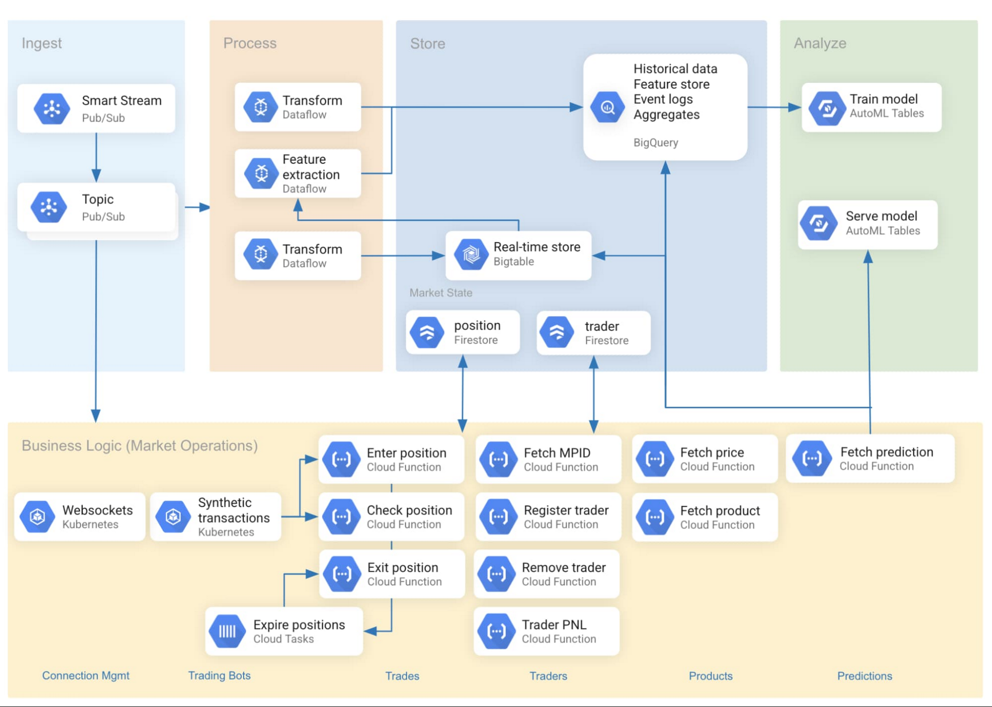
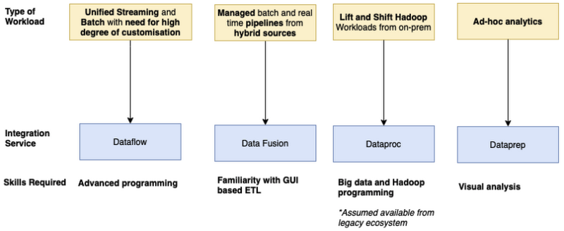
20210618 Orchestrating your data workloads in Google Cloud, EN
Services like Data Fusion, Dataflow and Dataproc are great for ingesting, processing and transforming your data. These services are designed to operate directly on big data and can build both batch and real time pipelines that support the performant aggregation (shuffling, grouping) and scaling of data. This is where you should build your data pipelines and you can use Composer to manage the execution of these services as part of a wider workflow.
Google Cloud’s first general purpose workflow orchestration tool was Cloud Composer.
However, if you want to process events or chain APIs in a serverless way—or have workloads that are bursty or latency-sensitive—we recommend Workflows.
Dataproc provides the ability for graphics processing units (GPUs) to be attached to the master and worker Compute Engine nodes in a Dataproc cluster. You can use these GPUs to accelerate specific workloads on your instances, such as machine learning and data processing.
Use the spark-bigquery-connector with Apache Spark to read and write data from and to BigQuery. This tutorial demonstrates a PySpark application that uses the spark-bigquery-connector.
Dataproc Serverless for Spark runs workloads within Docker containers. The container provides the runtime environment for the workload's driver and executor processes. By default, Dataproc Serverless for Spark uses a container image that includes the default Spark, Java, Python and R packages associated with a runtime release version. The Dataproc Serverless for Spark batches API allows you to use a custom container image instead of the default image. Typically, a custom container image adds Spark workload Java or Python dependencies not provided by the default container image. Important: Do not include Spark in your custom container image; Dataproc Serverless for Spark will mount Spark into the container at runtime.
When you submit your Spark workload, Dataproc Serverless for Spark can dynamically scale workload resources, such as the number of executors, to run your workload efficiently. Dataproc Serverless autoscaling is the default behavior, and uses Spark dynamic resource allocation to determine whether, how, and when to scale your workload.
Google is providing this collection of pre-implemented Dataproc templates as a reference and to provide easy customization for developers wanting to extend their functionality.
This repository contains Serverless Spark on GCP solution accelerators built around common use cases - helping data engineers and data scientists with Apache Spark experience ramp up faster on Serverless Spark on GCP.
This tutorial shows how to build a reusable pipeline that reads data from Cloud Storage, performs data quality checks, and writes to Cloud Storage.
Reusable pipelines have a regular pipeline structure, but you can change the configuration of each pipeline node based on configurations provided by an HTTP server. For example, a static pipeline might read data from Cloud Storage, apply transformations, and write to a BigQuery output table. If instead you want the transformation and BigQuery output table to change based on the Cloud Storage file that the pipeline reads, you create a reusable pipeline.
When Dataflow launches worker VMs, it uses Docker container images to launch containerized SDK processes on the workers. You can specify a custom container image instead of using one of the default Apache Beam images. When you specify a custom container image, Dataflow launches workers that pull the specified image. The following list includes reasons you might use a custom container:
Serverless VPC Access makes it possible for you to connect directly to your Virtual Private Cloud network from serverless environments such as Cloud Run, App Engine, or Cloud Functions. Configuring Serverless VPC Access allows your serverless environment to send requests to your VPC network using internal DNS and internal IP addresses (as defined by RFC 1918 and RFC 6598). The responses to these requests also use your internal network.
For your application to submit traces to Cloud Trace, it must be instrumented. You can instrument your code by using the Google client libraries. However, it's recommended that you use OpenTelemetry or OpenCensus to instrument your application. These are open source tracing packages. OpenTelemetry is actively in development and is the preferred package.
Each time series includes the metric kind (type MetricKind) for its data points. The kind of metric data tells you how to interpret the values relative to each other. Cloud Monitoring metrics are one of three kinds:
A gauge metric, in which the value measures a specific instant in time. For example, metrics measuring CPU utilization are gauge metrics; each point records the CPU utilization at the time of measurement. Another example of a gauge metric is the current temperature.
A delta metric, in which the value measures the change since it was last recorded. For example, metrics measuring request counts are delta metrics; each value records how many requests were received since the last data point was recorded.
A cumulative metric, in which the value constantly increases over time. For example, a metric for “sent bytes” might be cumulative; each value records the total number of bytes sent by a service at that time.
Log-based metrics derive metric data from the content of log entries. For example, you can use a log-based metric to count the number of log entries that contain a particular message or to extract latency information recorded in log entries. You can use log-based metrics in Cloud Monitoring charts and alerting policies.
# ist the project ID
gcloud config list project
[core]
project = qwiklabs-gcp-44776a13dea667a6

# set your Project ID
gcloud config set project <YOUR_PROJECT_ID>

# set it as an environment variable
export PROJECT_ID=$(gcloud config get-value project)
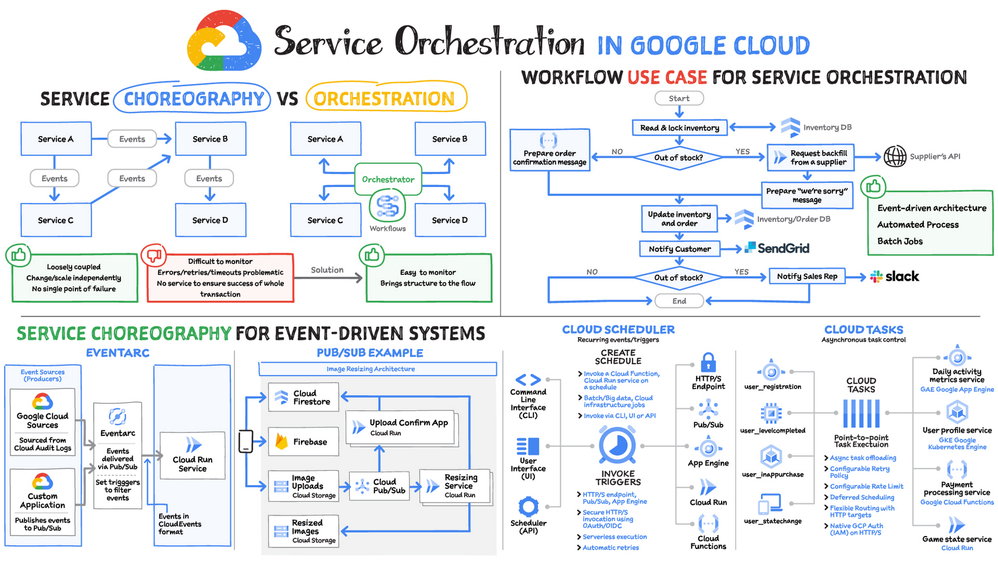
20211006 Service orchestration on Google Cloud, EN
Service Choreography - With service choreography, each service works independently and interacts with other services in a loosely coupled way through events. Loosely coupled events can be changed and scaled independently, which means there is no single point of failure. But, so many events flying around between services makes it quite hard to monitor. Business logic is distributed and spans across multiple services, so there is no single, central place to go for troubleshooting. There's no central source of truth to understand the system. Understanding, updating and troubleshooting are all distributed
Service Orchestration - To handle the monitoring challenges of choreography, developers need to bring structure to the flow of events, while retaining the loosely coupled nature of event-driven services. Using service orchestration, the services interact with each other via a central orchestrator that controls all interactions between the services. This orchestrator provides a high-level view of the business processes to track execution and troubleshoot issues. In Google Cloud, Workflows handles service orchestration.
Product
Description
Cloud Workflows
Suuport service orchestratio. Workflows is a fully-managed serverless service to orchestrate and automate Google Cloud and HTTP-based API services with serverless workflows. Workflows is particularly helpful with Google Cloud services that perform long-running operations, as Workflows will wait for them to complete, even if they take hours. With callbacks, Workflows can wait for external events for days or months. You can use either YAML or JSON to express your workflow.
Cloud Pub/Sub
Support service choreography. Pub/Sub enables services to communicate asynchronously, with latencies on the order of 100 milliseconds. Pub/Sub is used for messaging-oriented middleware for service integration or as a queue to parallelize tasks.
Cloud Eventarc
Support service choreography. Eventarc enables you to build event-driven architectures without having to implement, customize, or maintain the underlying infrastructure. Any service with Audit Log integration or any application that can send a message to a Pub/Sub topic can be event sources for Eventarc.
Cloud Task
Support service choreography. Cloud Tasks lets you separate out pieces of work that can be performed independently, outside of your main application flow, and send them off to be processed asynchronously using handlers that you create. Difference between Pub/Sub and Cloud Tasks. Pub/Sub supports implicit invocation: a publisher implicitly causes the subscribers to execute by publishing an event. Cloud Tasks is aimed at explicit invocation where the publisher retains full control of execution including specifying an endpoint where each message is to be delivered. Unlike Pub/Sub, Cloud Tasks provides tools for queue and task management including scheduling specific delivery times, rate controls, retries, and deduplication.
Cloud Scheduler
Support service choreography. With Cloud Scheduler, you set up scheduled units of work to be executed at defined times or regular intervals, commonly known as cron jobs. Cloud Scheduler can trigger a workflow (orchestration) or generate a Pub/Sub message (choreography). Cloud Scheduler uses cron scheduling to trigger the execution of HTTP-based services at a schedule you define.
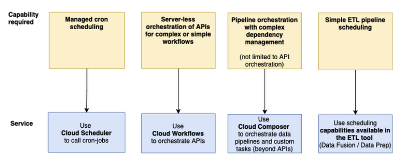
20210422 Choosing the right orchestrator in Google Cloud, EN
20210116 Eventarc: A unified eventing experience in Google Cloud | Google Cloud Blog
Eventarc provides an easier path to receive events not only from Pub/Sub topics but from a number of Google Cloud sources with its 'Audit Log' and Pub/Sub integration. Any service with Audit Log integration or any application that can send a message to a Pub/Sub topic can be event sources for Eventarc.
In Eventarc, different events from different sources are converted to 'CloudEvents' compliant events. CloudEvents is a specification for describing event data in a common way with the goal of consistency, accessibility and portability.
20201202 Better service orchestration with Workflows, EN
In Orchestration, a central service defines and controls the flow of communication between services. With centralization, it becomes easier to change and monitor the flow and apply consistent timeout and error policies.
In Choreography, each service registers for and emits events as they need. There’s usually a central event broker to pass messages around, but it does not define or direct the flow of communication. This allows services that are truly independent at the expense of less traceable and manageable flow and policies.
In orchestration vs choreography debate, there is no right answer. If you’re implementing a well-defined process with a bounded context, something you can picture with a flow diagram, orchestration is often the right solution. If you’re creating a distributed architecture across different domains, choreography can help those systems to work together.
After Lambda: Exactly-once processing in Cloud Dataflow,
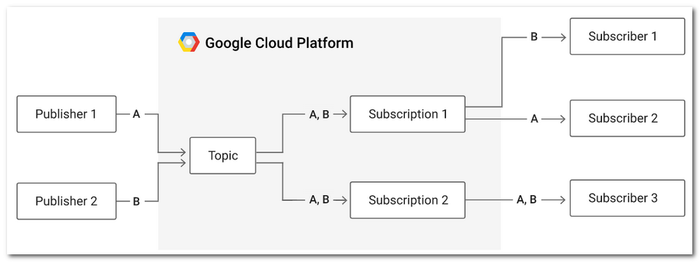
In this scenario, there are two publishers publishing messages on a single topic. There are two subscriptions to the topic.
The first subscription has two subscribers, meaning messages will be load-balanced across them, with each subscriber receiving a subset of the messages.
The second subscription has one subscriber that will receive all of the messages.
The bold letters represent messages. Message A comes from Publisher 1 and is sent to Subscriber 2 via Subscription 1, and to Subscriber 3 via Subscription 2. Message B comes from Publisher 2 and is sent to Subscriber 1 via Subscription 1 and to Subscriber 3 via Subscription 2.
Pub/Sub offers a broader range of features, per-message parallelism, global routing, and automatically scaling resource capacity.
Pub/Sub Lite can be as much as an order of magnitude less expensive, but offers lower availability and durability. In addition, Pub/Sub Lite requires you to manually reserve and manage resource capacity.
Retains unacknowledged messages in persistent storage for 7 days from the moment of publication. There is no limit on the number of retained messages. If subscribers don't use a subscription, the subscription expires. The default expiration period is 31 days.
Schema
Schema size (the definition field): 10KB
Publish request
10MB (total size); 1,000 messages
Message
Message size (the data field): 10MB; Attributes per message: 100; Attribute key size: 256 bytes; Attribute value size: 1024 bytes
Push outstanding messages
3,000 * N by default. 30,000 * N for subscriptions that acknowledge >99% of messages and average <1s of push request latency. N is the number of publish regions. For more information, see Using push subscriptions.
StreamingPull streams
10 MB/s per open stream
Pull/StreamingPull messages
The service might impose limits on the total number of outstanding StreamingPull messages per connection. If you run into such limits, increase the rate at which you acknowledge messages and the number of connections you use.
Quota mismatches
Quota mismatches can happen when published or received messages are smaller than 1000 bytes. For example:
If you publish 10 500-byte messages in separate requests, your publisher quota usage will be 10,000 bytes. This is because messages that are smaller than 1000 bytes are automatically rounded up to the next 1000-byte increment.
If you receive those 10 messages in a single pull response, your subscriber quota usage might be only 5 kB, since the actual size of each message is combined to determine the overall quota.
The inverse is also true. The subscriber quota usage might be greater than the publisher quota usage if you publish multiple messages in a single publish request or receive the messages in separate Pull requests.
Triggers actions at regular fixed intervals. You set up the interval when you create the cron job, and the rate does not change for the life of the job.
Triggers actions based on how the individual task object is configured. If the scheduleTime field is set, the action is triggered at that time. If the field is not set, the queue processes its tasks in a non-fixed order.
Setting rates
Initiates actions on a fixed periodic schedule. Once a minute is the most fine-grained interval supported.
Initiates actions based on the amount of traffic coming through the queue. You can set a maximum rate when you create the queue, for throttling or traffic smoothing purposes, up to 500 dispatches per second.
Naming
Except for the time of execution, each run of a cron job is exactly the same as every other run of that cron job.
Each task has a unique name, and can be identified and managed individually in the queue.
Handling failure
If the execution of a cron job fails, the failure is logged. If retry behavior is not specifically configured, the job is not rerun until the next scheduled interval.
If the execution of a task fails, the task is re-tried until it succeeds. You can limit retries based on the number of attempts and/or the age of the task, and you can control the interval between attempts in the configuration of the queue.
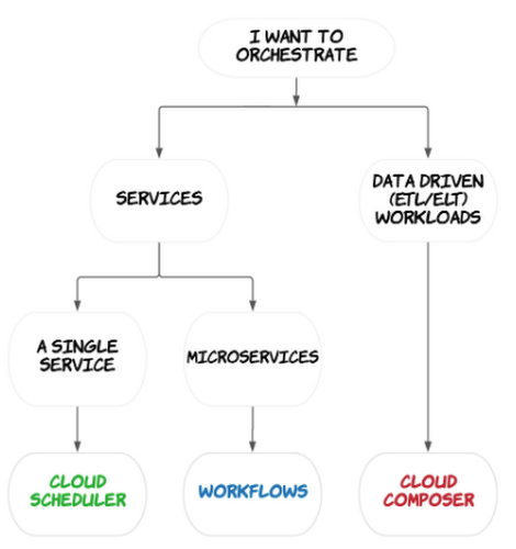
Workflows orchestrates multiple HTTP-based services into a durable and stateful workflow. It has low latency and can handle a high number of executions. It's also completely serverless.
Workflows is great for chaining microservices together, automating infrastructure tasks like starting or stopping a VM, and integrating with external systems. Workflows connectors also support simple sequences of operations in Google Cloud services such as Cloud Storage and BigQuery.
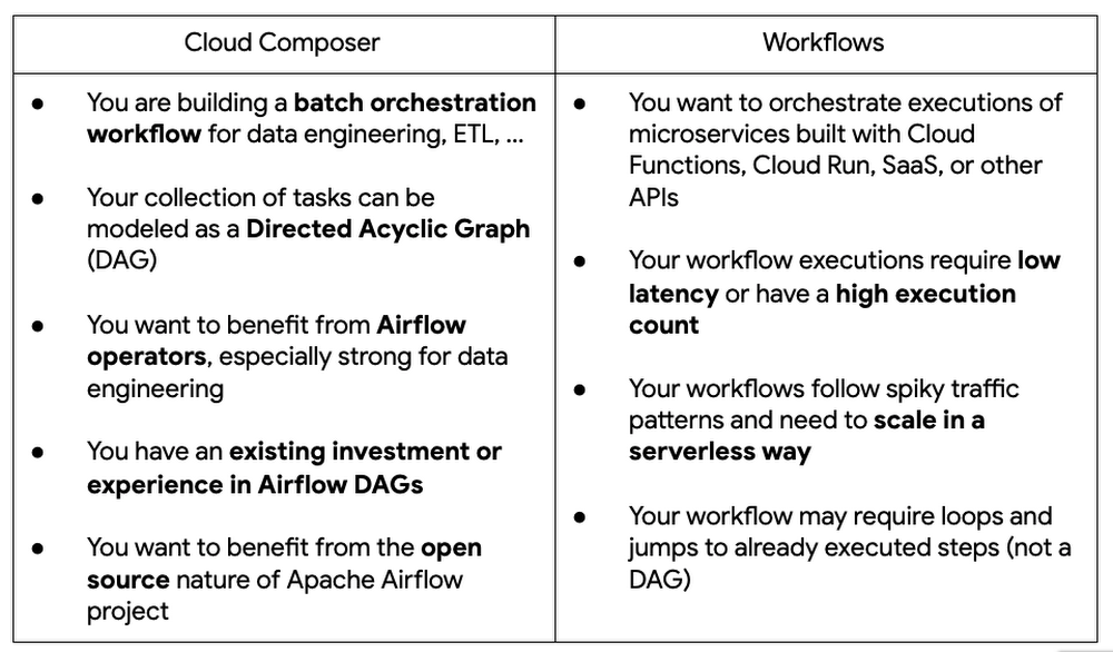
Cloud Composer is designed to orchestrate data driven workflows (particularly ETL/ELT). It's built on the Apache Airflow project, but Cloud Composer is fully managed. Cloud Composer supports your pipelines wherever they are, including on-premises or across multiple cloud platforms. All logic in Cloud Composer, including tasks and scheduling, is expressed in Python as Directed Acyclic Graph (DAG) definition files.
Cloud Composer is best for batch workloads that can handle a few seconds of latency between task executions. You can use Cloud Composer to orchestrate services in your data pipelines, such as triggering a job in BigQuery or starting a Dataflow pipeline. You can use pre-existing operators to communicate with various services, and there are over 150 operators for Google Cloud alone.
Detailed feature comparison
Feature
Workflows
Cloud Composer
Syntax
Workflows syntax in YAML or JSON format
Python
State model
Imperative flow control
Declarative DAG with automatic dependency resolution


GSP246: Predict Taxi Fare with a BigQuery ML Forecasting Model
Linear Regression with Pyspark in 10 steps.
20221205 MLOps at Walgreens Boots Alliance With Databricks Lakehouse Platform - The Databricks Blog, EN