At the validation stage, models with few or no hyperparameters are straightforward to validate and tune. Thus, a relatively small dataset should suffice.
In contrast, models with multiple hyperparameters require enough data to validate likely inputs. CV might be helpful in these cases, too. Generally, apportioning 80 percent of the records to train, 10 percent to validate, and 10 percent to test scenarios ought to be a reasonable initial split.
Variables of interest in an experiment (those that are measured or observed) are called response or dependent variables. Other variables in the experiment that affect the response and can be set or measured by the experimenter are called predictor, explanatory, or independent variables.
For example, you might want to determine the recommended baking time for a cake recipe or provide care instructions for a new hybrid plant.
| Subject | Possible predictor variables | Possible response variables |
|---|---|---|
| Cake recipe | Baking time, oven temperature | Moisture of the cake, thickness of the cake |
| Plant growth | Amount of light, pH of the soil, frequency of watering | Size of the leaves, height of the plant |
A continuous predictor variable is sometimes called a covariate and a categorical predictor variable is sometimes called a factor. In the cake experiment, a covariate could be various oven temperatures and a factor could be different ovens.
Usually, you create a plot of predictor variables on the x-axis and response variables on the y-axis.
-
2014 Machine Learning: The High Interest Credit Card of Technical Debt, https://research.google/pubs/pub43146/
Machine learning offers a fantastically powerful toolkit for building complex systems quickly. This paper argues that it is dangerous to think of these quick wins as coming for free. Using the framework of technical debt, we note that it is remarkably easy to incur massive ongoing maintenance costs at the system level when applying machine learning. The goal of this paper is highlight several machine learning specific risk factors and design patterns to be avoided or refactored where possible. These include boundary erosion, entanglement, hidden feedback loops, undeclared consumers, data dependencies, changes in the external world, and a variety of system-level anti-patterns.

- A logical, reasonably standardized, but flexible project structure for doing and sharing data science work, https://drivendata.github.io/cookiecutter-data-science/
├── LICENSE
├── Makefile           <- Makefile with commands like `make data` or `make train`
├── README.md          <- The top-level README for developers using this project.
├── data
│   ├── external       <- Data from third party sources.
│   ├── interim        <- Intermediate data that has been transformed.
│   ├── processed      <- The final, canonical data sets for modeling.
│   └── raw            <- The original, immutable data dump.
│
├── docs               <- A default Sphinx project; see sphinx-doc.org for details
│
├── models             <- Trained and serialized models, model predictions, or model summaries
│
├── notebooks          <- Jupyter notebooks. Naming convention is a number (for ordering),
│                         the creator's initials, and a short `-` delimited description, e.g.
│                         `1.0-jqp-initial-data-exploration`.
│
├── references         <- Data dictionaries, manuals, and all other explanatory materials.
│
├── reports            <- Generated analysis as HTML, PDF, LaTeX, etc.
│   └── figures        <- Generated graphics and figures to be used in reporting
│
├── requirements.txt   <- The requirements file for reproducing the analysis environment, e.g.
│                         generated with `pip freeze > requirements.txt`
│
├── setup.py           <- Make this project pip installable with `pip install -e`
├── src                <- Source code for use in this project.
│   ├── __init__.py    <- Makes src a Python module
│   │
│   ├── data           <- Scripts to download or generate data
│   │   └── make_dataset.py
│   │
│   ├── features       <- Scripts to turn raw data into features for modeling
│   │   └── build_features.py
│   │
│   ├── models         <- Scripts to train models and then use trained models to make
│   │   │                 predictions
│   │   ├── predict_model.py
│   │   └── train_model.py
│   │
│   └── visualization  <- Scripts to create exploratory and results oriented visualizations
│       └── visualize.py
│
└── tox.ini            <- tox file with settings for running tox; see tox.readthedocs.io
-
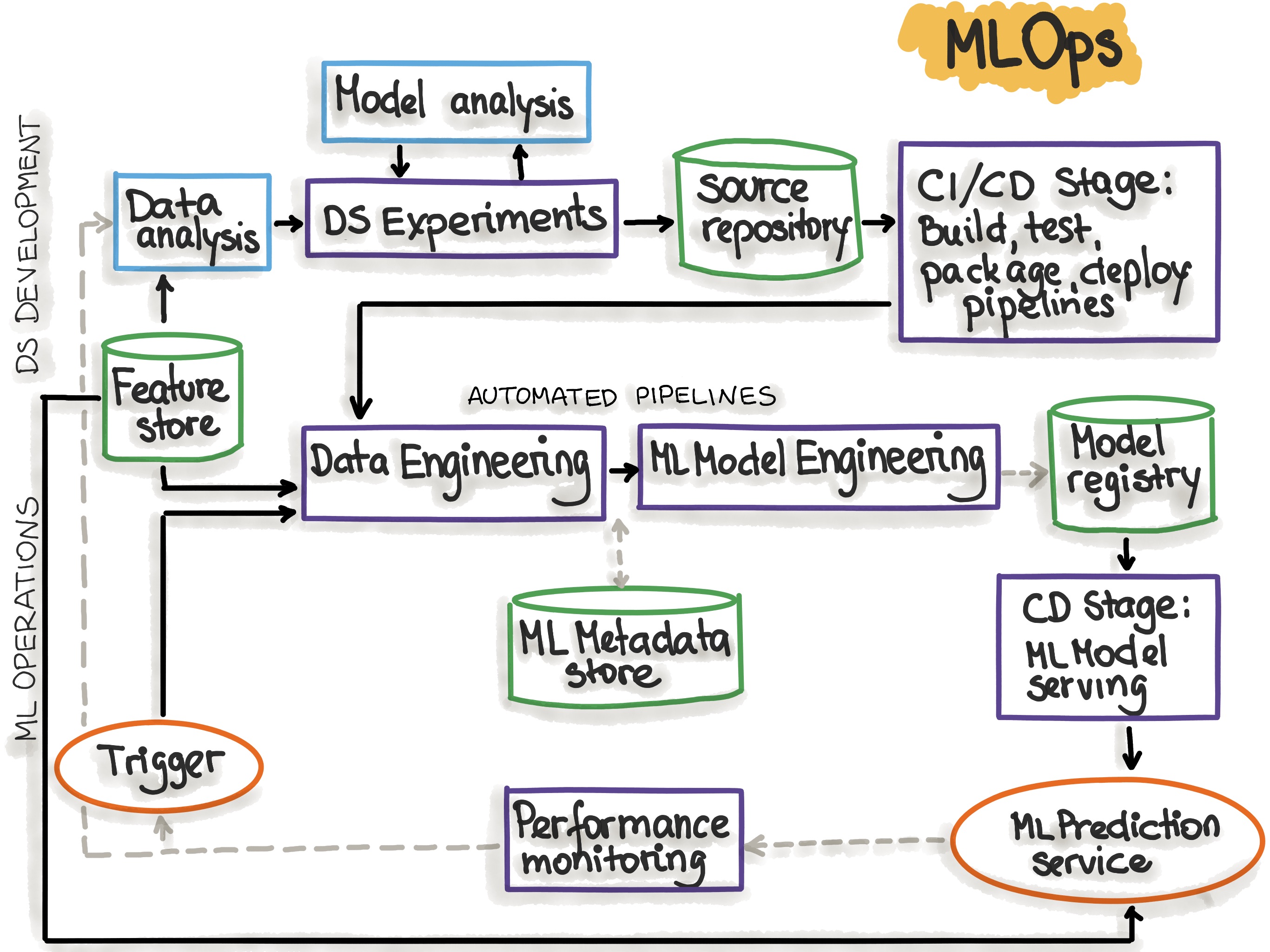
With Machine Learning Model Operationalization Management (MLOps), we want to provide an end-to-end machine learning development process to design, build and manage reproducible, testable, and evolvable ML-powered software.
-
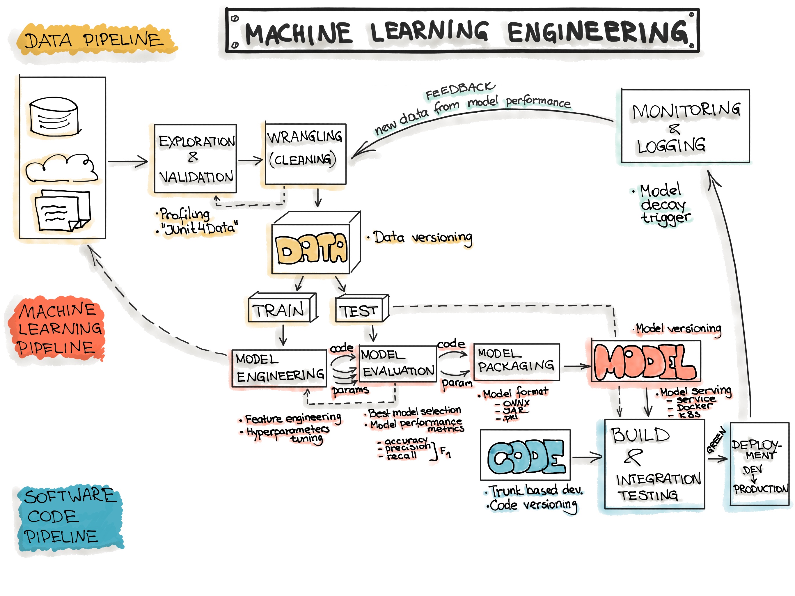
An Overview of the End-to-End Machine Learning Workflow, https://ml-ops.org/content/end-to-end-ml-workflow
- Data Engineering
- Data Ingestion - Collecting data by using various frameworks and formats, such as Spark, HDFS, CSV, etc. This step might also include synthetic data generation or data enrichment.
- Exploration and Validation - Includes data profiling to obtain information about the content and structure of the data. The output of this step is a set of metadata, such as max, min, avg of values. Data validation operations are user-defined error detection functions, which scan the dataset in order to spot some errors.
- Data Wrangling (Cleaning) - The process of re-formatting particular attributes and correcting errors in data, such as missing values imputation.
- Data Labeling - The operation of the Data Engineering pipeline, where each data point is assigned to a specific category.
- Data Splitting - Splitting the data into training, validation, and test datasets to be used during the core machine learning stages to produce the ML model.
- Model Engineering
- Model Training - The process of applying the machine learning algorithm on training data to train an ML model. It also includes feature engineering and the hyperparameter tuning for the model training activity.
- Model Evaluation - Validating the trained model to ensure it meets original codified objectives before serving the ML model in production to the end-user.
- Model Testing - Performing the final “Model Acceptance Test” by using the hold backtest dataset.
- Model Packaging - The process of exporting the final ML model into a specific format (e.g. PMML, PFA, or ONNX), which describes the model, in order to be consumed by the business application.
- Model Deployment
- Model Serving - The process of addressing the ML model artifact in a production environment.
- Model Performance Monitoring - The process of observing the ML model performance based on live and previously unseen data, such as prediction or recommendation. In particular, we are interested in ML-specific signals, such as prediction deviation from previous model performance. These signals might be used as triggers for model re-training.
- Model Performance Logging - Every inference request results in the log-record.
- Data Engineering
-
MLOps Principles, https://ml-ops.org/content/mlops-principles#summary-of-mlops-principles-and-best-practices
Summary of MLOps Principles and Best Practices:
| MLOps Principles | Data | ML Model | Code |
|---|---|---|---|
| Versioning | 1) Data preparation pipelines 2) Features store 3) Datasets 4) Metadata |
1) ML model training pipeline 2) ML model (object) 3) Hyperparameters 4) Experiment tracking |
1) Application code 2) Configurations |
| Testing | 1) Data Validation (error detection) 2) Feature creation unit testing |
1) Model specification is unit tested 2) ML model training pipeline is integration tested 3) ML model is validated before being operationalized 4) ML model staleness test (in production) 5) Testing ML model relevance and correctness 6) Testing non-functional requirements (security, fairness, interpretability) |
1) Unit testing 2) Integration testing for the end-to-end pipeline |
| Automation | 1) Data transformation 2) Feature creation and manipulation 1) Data engineering pipeline 2) ML model training pipeline 3) Hyperparameter/Parameter selection |
1) ML model deployment with CI/CD 2) Application build |
|
| Reproducibility | 1) Backup data 2) Data versioning 3) Extract metadata 4) Versioning of feature engineering |
1) Hyperparameter tuning is identical between dev and prod 2) The order of features is the same 3) Ensemble learning: the combination of ML models is same 4)The model pseudo-code is documented |
1) Versions of all dependencies in dev and prod are identical 2) Same technical stack for dev and production environments 3) Reproducing results by providing container images or virtual machines |
| Deployment | 1) Feature store is used in dev and prod environments |
1) Containerization of the ML stack 2) REST API 3) On-premise, cloud, or edge |
1) On-premise, cloud, or edge |
| Monitoring | 1) Data distribution changes (training vs. serving data) 2) Training vs serving features |
1) ML model decay 2) Numerical stability 3) Computational performance of the ML model |
1) Predictive quality of the application on serving data |
-
MLOps Stack Canvas, https://ml-ops.org/content/mlops-stack-canvas
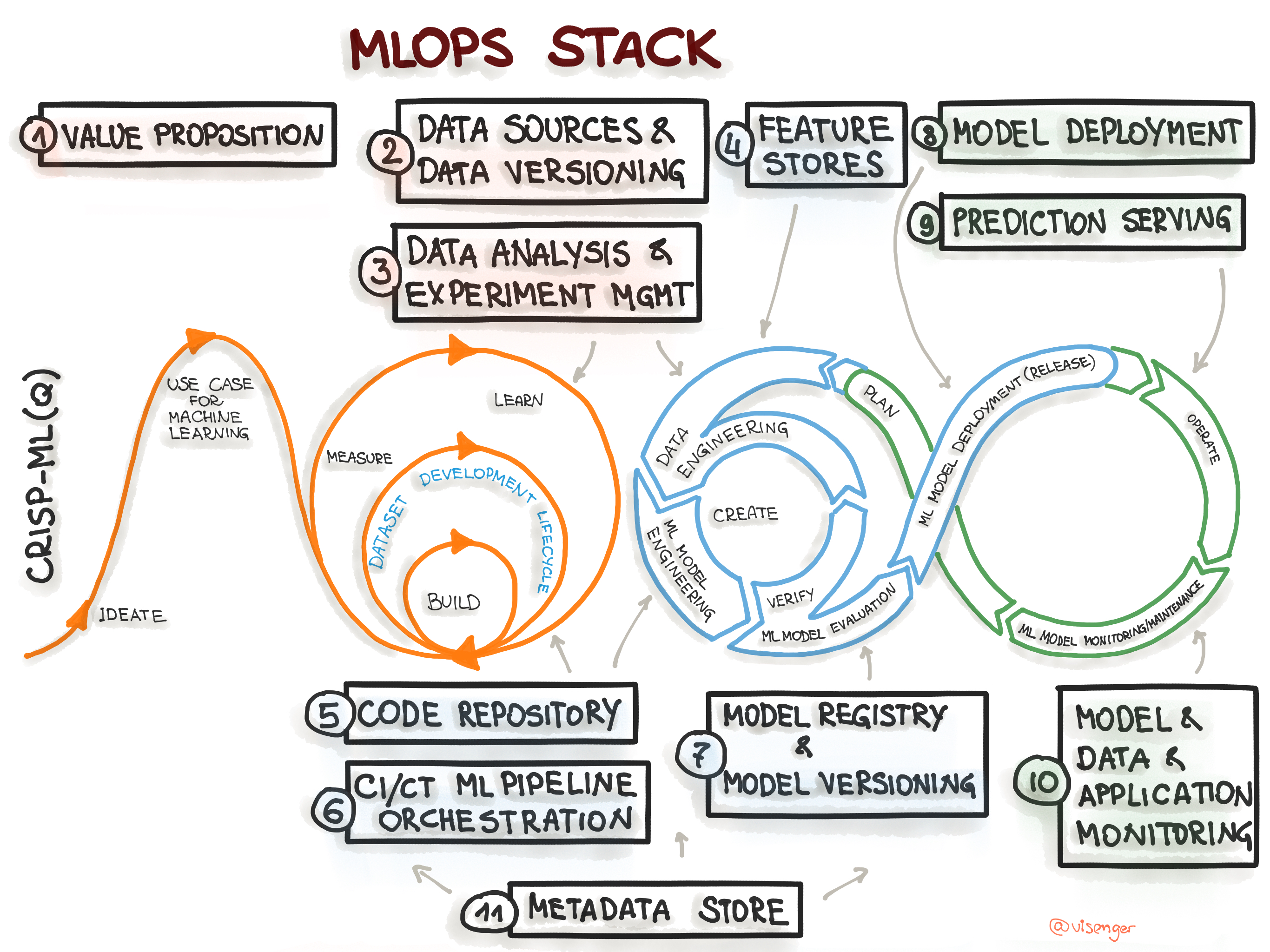
To specify an architecture and infrastructure stack for Machine Learning Operations, we suggest a general MLOps Stack Canvas framework designed to be application- and industry-neutral. We align to the CRISP-ML(Q) model and describe the eleven components of the MLOps stack and line them up along with the ML Lifecycle and the “AI Readiness” level to select the right amount of MLOps processes and technlogy components.
Figure 1. Mapping the CRISP-ML(Q) process model to the MLOps stack.
-
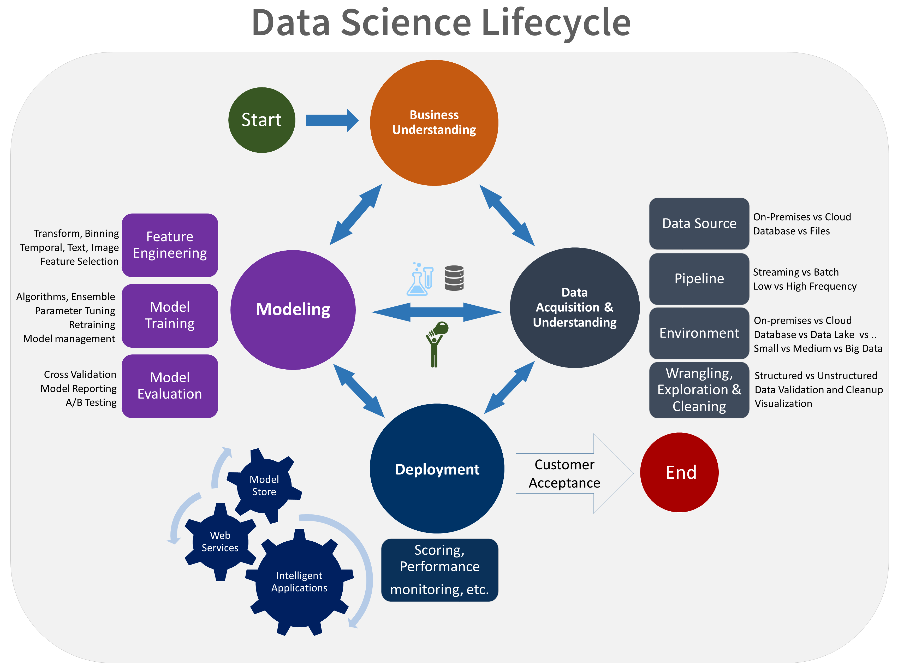
What is the Team Data Science Process, https://docs.microsoft.com/en-us/azure/machine-learning/team-data-science-process/overview
-
https://docs.aws.amazon.com/machine-learning/latest/dg/the-machine-learning-process.html
ML Processes:
- Analyze your data
- Split data into training and evaluation datasources
- Shuffle your training data
- Process features
- Train the model
- Select model parameters
- Evaluate the model performance
- Feature selection
- Set a score threshold for prediction accuracy
- Use the model


