Simulate and plot Poisson and Negative Binomial distributions in R

simulate_distributions.R

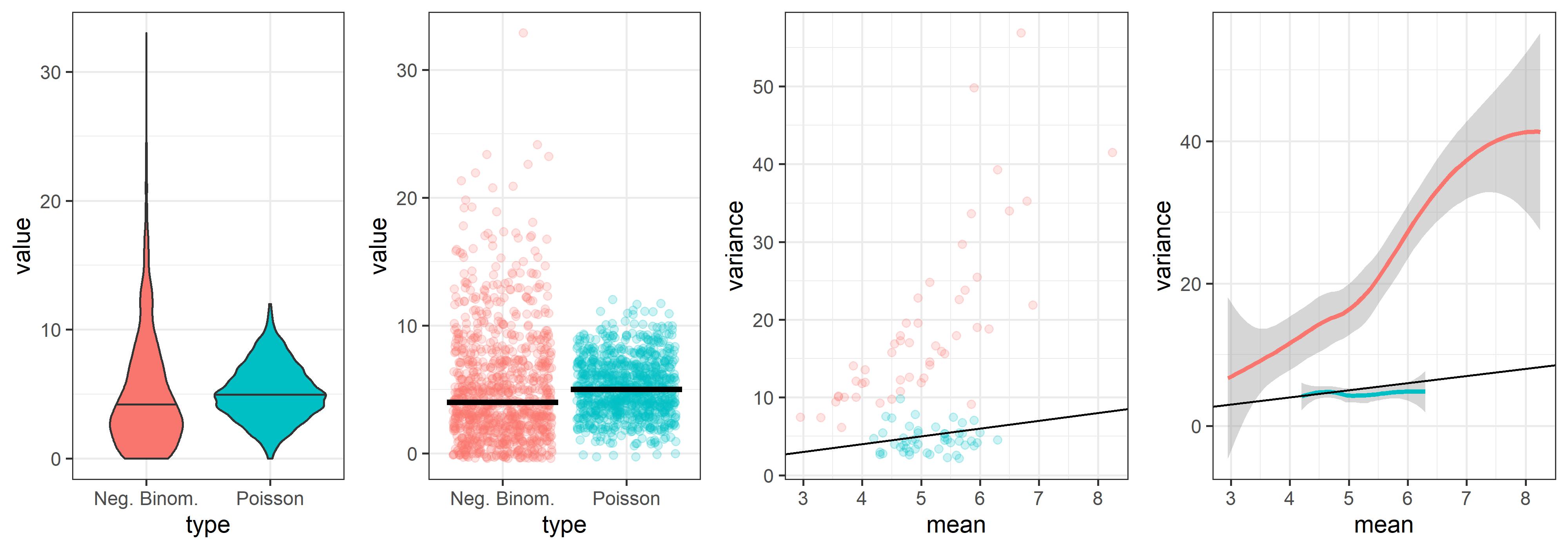
#!/usr/bin/env R

# Author: Sean Maden
#
# Simulate Poisson and Negative Binomial distributions, plotting the point 
# values and mean-variance relationships.
#


# load dependencies
libv <- c("ggplot2", "gridExtra")
sapply(libv, library, character.only = TRUE)

# set plot parameters
pt.alpha <- 0.2
jpg.width = 10
jpg.height = 3.5
num <- 5 # layout scale value
jpg.fname <- "dist-examples.jpeg"

# set simulation parameters
seed.num <- 0
num.points <- 1e3 # total data points
num.groups <- 50 # analogous to genes
set.seed(seed.num)

# simulate new data
set.seed(seed.num)
rn <- rnbinom(n = num.points, size = 2, mu = 5)
rp <- rpois(num.points, lambda = 5)
mrn <- matrix(rn, nrow = num.groups)
mrp <- matrix(rp, nrow = num.groups)

# get violin plots
dfp1 <- data.frame(value = rn); dfp1$type <- "Neg. Binom."
dfp2 <- data.frame(value = rp); dfp2$type <- "Poisson"
dfp.pt <- rbind(dfp1, dfp2)
plot1 <- ggplot(dfp.pt, aes(x = type, y = value, fill = type)) + 
  geom_violin(draw_quantiles = 0.5) + theme_bw() +
  theme(legend.position = "none")

# get jitter plots
dfp1 <- data.frame(value = rn); dfp1$type <- "Neg. Binom."
dfp2 <- data.frame(value = rp); dfp2$type <- "Poisson"
dfp.pt <- rbind(dfp1, dfp2)
plot2 <- ggplot(dfp.pt, aes(x = type, y = value, color = type)) + 
  geom_jitter(alpha = pt.alpha) + theme_bw() +
  theme(legend.position = "none") +
  stat_summary(fun = "median", color = "black", geom = "crossbar")

# get mean-variance plots
dfp1 <- data.frame(mean = rowMeans(mrn),
                   variance = rowVars(mrn))
dfp1$type <- "Neg. Binom."
dfp2 <- data.frame(mean = rowMeans(mrp),
                   variance = rowVars(mrp))
dfp2$type <- "Poisson"
dfp.mv <- rbind(dfp1, dfp2)
plot3 <- ggplot(dfp.mv, aes(x = mean, y = variance, group = type, color = type)) + 
  geom_point(alpha = pt.alpha) + geom_abline(slope = 1, intercept = 0) +
  theme_bw() + theme(legend.position = "none")
plot4 <- ggplot(dfp.mv, aes(x = mean, y = variance, group = type, color = type)) + 
  geom_smooth() + geom_abline(slope = 1, intercept = 0) +
  theme_bw() + theme(legend.position = "none")

# save composite plots
lm <- matrix(c(rep(1, num), rep(2, num), 
               rep(3, num+1), rep(4, num+1)), nrow = 1)
jpeg(jpg.fname, width = jpg.width, height = jpg.height, 
     units = "in", res = 400)
grid.arrange(plot1, plot2, plot3, plot4, nrow = 1, layout_matrix = lm)
dev.off()

Plot output