installing flow* on fedora

gistfile1.md

Getting the software

First download Flow*, https://flowstar.org/dowloads/

At the time of writing the latest release is v2.1.0 from march 2017.

The following installation instructions were tested on a Dell 9575 laptop running Fedora 31.

Installing the dependencies

Install MPFR following installation instructions from https://www.mpfr.org/mpfr-current/mpfr.html#Installing-MPFR.

Also, install the following packages:

$ sudo dnf install mpfr-devel
$ sudo dnf install gmp-devel
$ sudo dnf install gsl
$ sudo dnf install gsl-devel
$ sudo dnf install glpk-devel
$ sudo dnf install bison
$ sudo dnf install flex
$ sudo dnf install gnuplot

Unfortunately this was not enough and I had add the library libfmp.so.6 manually like so:

$ sudo cp /home/mforets/Tools/julia-1.3.0-rc4-linux-x86_64/julia-1.3.0-rc4/lib/julia/libmpfr.so.6 /usr/lib64/

Compiling Flow*

Then go to the folder where you have Flow*'s Makefile and do $ make. If the installation is successful, you should now have an executable file flowstar in your working directory.

Testing Flow*

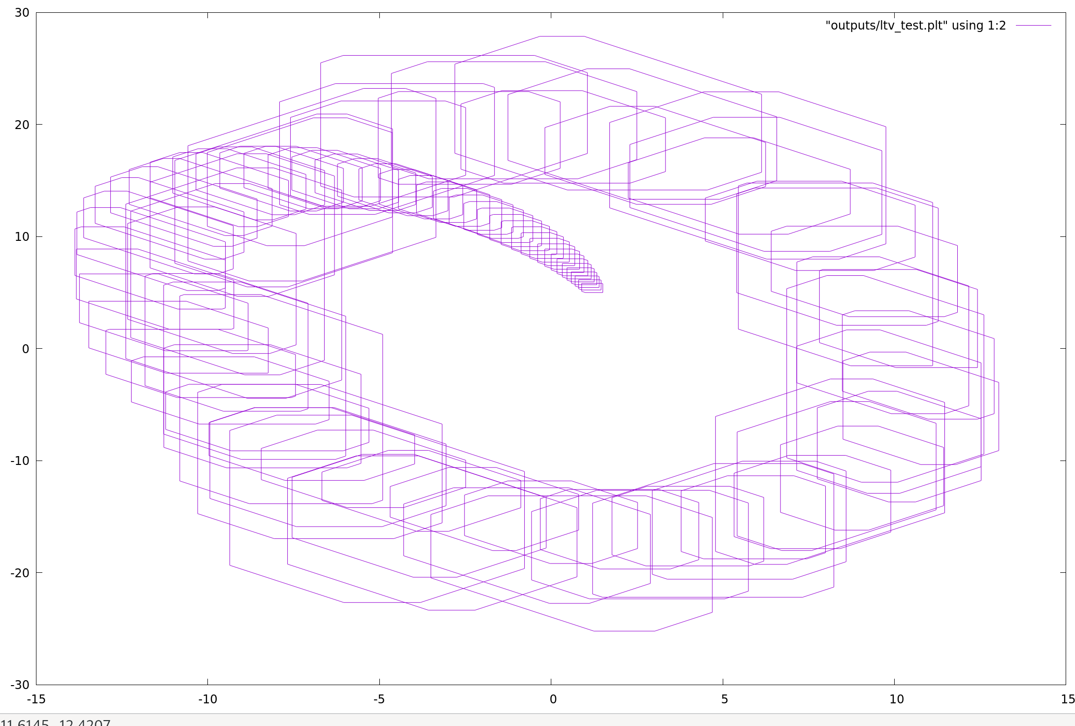
If everything is fine, you should be able to run Flow* on some model. Below we try the two-dimensional linear time-varying system from https://flowstar.org/benchmarks/2-dimensional-ltv-system/

First we copy the model to a file named ltv_2D.model and run flowstar:

$ ./flowstar < models/ltv_2D.model 
time = 0.050000,	step = 0.050000,	order = 8
time = 0.100000,	step = 0.050000,	order = 8
...
Computation completed: 100 flowpipe(s) computed.
Total time cost: 0.274921 seconds.

Preparing for plotting and dumping...
%100
Done.
Generating the plot file...
%100
Done.
Writing the flowpipe(s)...
Done.

This creates two output files in the output folder, one containing the output, and another containing plot data.

To plot the data we use gnuplot.

$ gnuplot

gnuplot> plot "outputs/ltv_test.plt" using 1:2 with lines

creates