Linear regression with gradient descent in R.

readme.md

Linear Regression with Gradient Descent in R

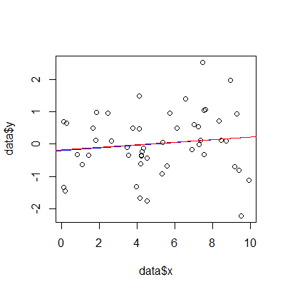
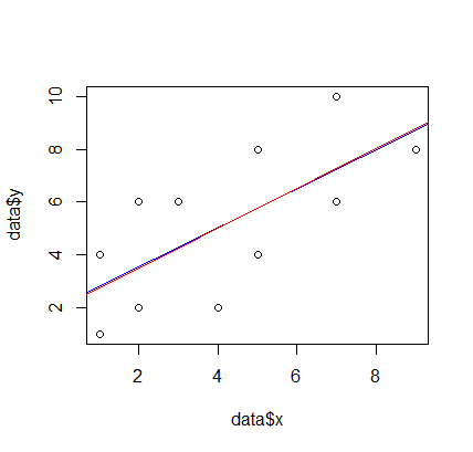
An example of manually calculating a linear regression for a single variable (x, y) using gradient descent. This demonstrates a basic machine learning linear regression.

In the outputs, compare the values for intercept and slope from the built-in R lm() method with those that we calculate manually with gradient descent. The plots show how close the red and blue lines overlap.

linear-regression.R

#
# An example of calculating linear regression with gradient descent for a single variable.
# Kory Becker
# 1/31/2020
#

# Calculate linear regression with gradient descent.
linearRegression <- function(x, y, alpha, iterations) {
  # initialize coefficients
  theta <- matrix(c(0,0), nrow=2)
  
  # add a column of 1's for the intercept coefficient
  X <- cbind(1, matrix(x))
  
  # gradient descent
  for (i in 1:num_iters) {
    error <- (X %*% theta - y)
    delta <- t(X) %*% error / length(y)
    theta <- theta - alpha * delta
  }
  
  list(intercept=theta[1], slope=theta[2])
}

data1 <- list(x=c(1, 2, 4, 5, 7, 9, 1, 2, 3, 5, 7), y=c(1, 2, 2, 4, 6, 8, 4, 6, 6, 8, 10))
data2 <- list(x=runif(50, 0, 10), y=rnorm(50))

demo <- function(data) {
  # Plot grid.
  abline(h = 0:10, v = 0:8, col = "lightgray", lty=3)
  
  # Plot points.
  plot(data)
  
  # f(x) <- m*x + b
  # h(x) <- w0 + w1*x
  
  # Calculate linear model.
  model1 <- lm(y ~ x, data)

  # Plot regression line by intercept and slope.
  abline(model1$coefficients[1], model1$coefficients[2], col='blue')
  
  model2 <- linearRegression(data$x, data$y, 0.01, 100)
  
  # Plot regression line by intercept and slope.
  abline(model2$intercept, model2$slope, col='red')
  
  list(model1=model1, model2=model2)
}

models <- demo(data1)
print(models)

output1.txt

$model1

Call:
lm(formula = y ~ x, data = data)

Coefficients:
(Intercept)            x  
     2.1091       0.7348  


$model2
$model2$intercept
[1] 1.971589

$model2$slope
[1] 0.7590041

output2.txt

$model1

Call:
lm(formula = y ~ x, data = data)

Coefficients:
(Intercept)            x  
   -0.19325      0.04124  


$model2
$model2$intercept
[1] -0.1740673

$model2$slope
[1] 0.03834414