Authors : Alex Krizhevsky, Ilya Sutskever, and Geoffrey Hinton
This was one of the most influential publication in the field of Computer Vision.This model won the ILSVRC 2012 Competition.
1.Trained the network on ImageNet data which contained over 15 million images form over 22,000 categories.
2. This paper uses ReLU activation function for non linearity. ReLU was found to decresase the run time of training , as it was faster than conventional tanh function.
3. Dropout was implemented to reduce the effect of overfitting.
4. Data Augumentation technique was used that consisted of image translation, patch extraction and image reflection.
5. Stochastic Gradient Descent was used as optimizer with momentum and weight decay.
6. This model was trained on GTX 580 GPUs for aroung 6 days.
Imagenet is a dataset of over 15 million images belonging to roughlt 22,000 categories.The images were collected from the web and labeled by human labelers using Amazon’s Mechanical Turk crowd-sourcing tool. Starting in 2010, as part of the Pascal Visual Object Challenge, an annual competition called the ImageNet Large-Scale Visual Recognition Challenge (ILSVRC) has been held. ILSVRC uses a subset of ImageNet with roughly 1000 images in each of 1000 categories. In all, there are roughly 1.2 million training images, 50,000 validation images, and 150,000 testing images.
Due to computational reasons, we will use CIFAR-10 Dataset in this paper implementation.
The standard way of implementing neuron's output before this paper was to use tanh activation.
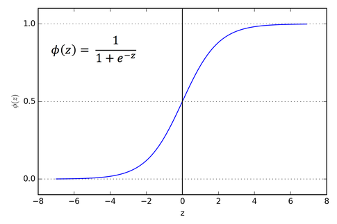
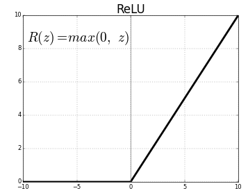
It was observed that the training time of tanh activation function was bigger than that of ReLU activation during backpropagation step in gradient descent optimization.
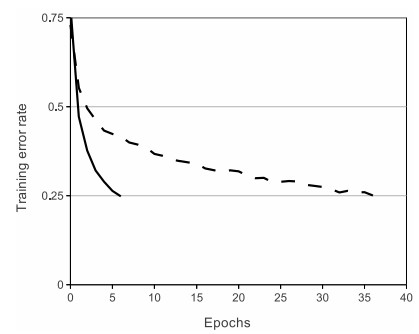
solid line - ReLU
dashed line - tanh
import numpy as np

def ReLU(x):
  return abs(x) * (x > 0)

x = np.array([1,-1, -0.5, 0.32])
ReLU(x)
array([1. , 0. , 0. , 0.32])
import torch

relu = torch.nn.ReLU()

x = torch.tensor(x) # x = numpy array of [1,-1, -0.5, 0.32]
relu(x)
tensor([1.0000, 0.0000, 0.0000, 0.3200], dtype=torch.float64)
Relu has this desirable property that they do not need input normalization to prevent them from saturating. Learning will occur through ReLU even if some of the training data predoce positive input. However it is still observed that Local Response Normalization helps in generalization.
import torch.nn as nn

class LRN(nn.Module):
  def __init__(self, size, alpha=1e-4, beta=0.75, k=1):
    super(LRN, self).__init__()
    self.avg = nn.AvgPool3d(kernel_size =(size,1,1), stride=1, padding=int((size-1)/2))
    self.alpha = alpha
    self.beta = beta
    self.k = k

  def forward(self, x):
    deno = x.pow(2).unsqueeze(1)
    deno = self.avg(deno).squeeze(1)
    deno = deno.mul(self.alpha).add(self.k).pow(self.beta)
    x = x.div(deno)
    return x


x = torch.randn( 20,3, 10, 10)
lrn = nn.LocalResponseNorm(2)
lrn(x).size()
torch.Size([20, 3, 10, 10])
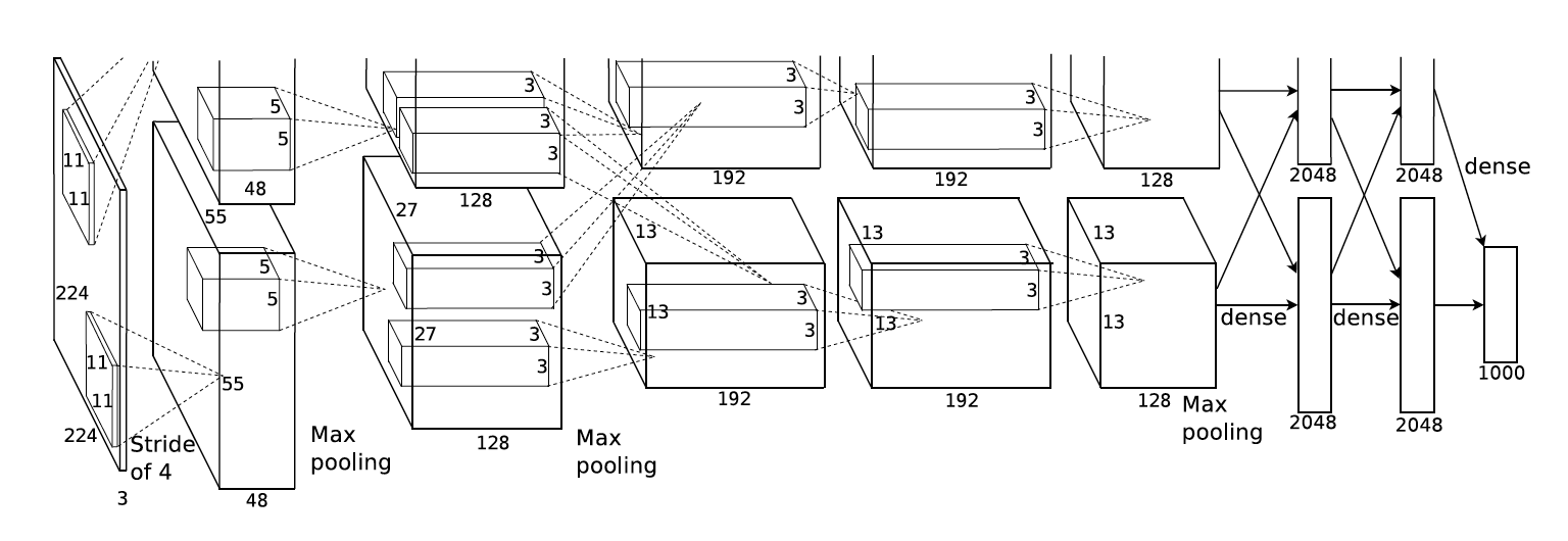
class AlexNet(nn.Module):
  def __init__(self, classes=1000):
    super(AlexNet, self).__init__()
    self.features = nn.Sequential(
            nn.Conv2d(3, 64, kernel_size=11, stride=4, padding=2),
            nn.ReLU(inplace=True),
            nn.MaxPool2d(kernel_size=3, stride=2),
            nn.Conv2d(64, 192, kernel_size=5, padding=2),
            nn.ReLU(inplace=True),
            nn.MaxPool2d(kernel_size=3, stride=2),
            nn.Conv2d(192, 384, kernel_size=3, padding=1),
            nn.ReLU(inplace=True),
            nn.Conv2d(384, 256, kernel_size=3, padding=1),
            nn.ReLU(inplace=True),
            nn.Conv2d(256, 256, kernel_size=3, padding=1),
            nn.ReLU(inplace=True),
            nn.MaxPool2d(kernel_size=3, stride=2),
    )
    self.classifier = nn.Sequential(
            nn.Dropout(),
            nn.Linear(256 * 6 * 6, 4096),
            nn.ReLU(inplace=True),
            nn.Dropout(),
            nn.Linear(4096, 4096),
            nn.ReLU(inplace=True),
            nn.Linear(4096, classes),
    )
  def forward(self, x):
      x = self.features(x)
      x = x.view(x.size(0), 256 * 6 * 6)
      x = self.classifier(x)
      return x


x = torch.randn(1, 3, 224, 224).uniform_(0, 1)
alexnet = AlexNet()
alexnet(x).size()
torch.Size([1, 1000])
The easiest way to avoid over fitting is to increase the data size, so that the model can learn more generalized features of the data.
But getting more data is always not an easy task , so one of the way of getting more data is to artificially generate more data from the given data.
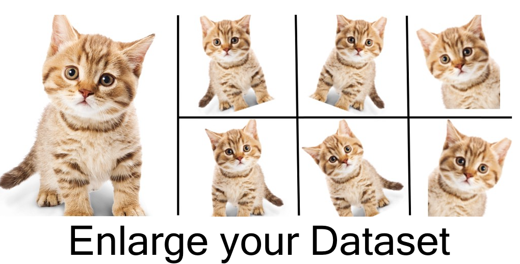

There are many types of data augmentation techniques available
-
Flip (horizontal and vertical)
-
Rotation
-
Scaling
-
Crop
-
Translation
-
Gaussian noise
from skimage import io
import matplotlib.pyplot as plt

image = io.imread('https://cdn3.bigcommerce.com/s-nadnq/product_images/uploaded_images/20.jpg')

plt.imshow(image)
plt.grid(False)
plt.axis('off')
plt.show()

import random
from scipy import ndarray
import skimage as sk
from skimage import transform
from skimage import util

def random_rotation(image_array: ndarray):
    random_degree = random.uniform(-25, 25)
    return sk.transform.rotate(image_array, random_degree)

def random_noise(image_array: ndarray):
    return sk.util.random_noise(image_array)

def horizontal_flip(image_array: ndarray):
    return image_array[:, ::-1]

def vertical_flip(image_array: ndarray):
    return image_array[::-1, :]
This technique reduces complex co-adaptations of neurons, since a neuron cannot rely on the presence of particular other neurons. It is, therefore, forced to learn more robust features that are useful in conjunction with many different random subsets of the other neurons. At test time, we use all the neurons but multiply their outputs by 0.5, which is a reasonable approximation to taking the geometric mean of the predictive distributions produced by the exponentially-many dropout networks.

def dropout(X, drop_probability):
    keep_probability = 1 - drop_probability
    mask = np.random.uniform(0, 1.0, X.shape) < keep_probability
    if keep_probability > 0.0:
        scale = (1/keep_probability)
    else:
        scale = 0.0
    return mask * X * scale

x = np.random.randn(3,3)
dropout(x, 0.3)
array([[ 0.        ,  2.12769017, -1.95883643],
       [ 0.05583112, -0.51280684,  0.        ],
       [-1.64030713,  3.15857694,  1.13236446]])
import torch

x = np.random.randn(3,3)
x_tensor = torch.from_numpy(x)

dropout = torch.nn.Dropout(0.5)
dropout(x_tensor)
tensor([[ 0.9667,  0.0000,  2.1510],
        [ 1.4301,  0.0000,  1.4544],
        [-0.0000,  1.3651, -0.0000]], dtype=torch.float64)
Gradient Descent optimizer with momentim of 0.9 and weight decay of 0.0005 is used. Batch size of 128.
Weight in each layer is initialized from a zero mean Gaussian Distribution with standard deviation 0.01. bias was initialized with 1.
manual adjusting of learning rates and lr was reduced when loss stopped increasing.
weights = np.random.normal(loc=0.0, scale=0.01, size=(3,3))
weights
array([[-0.00723783, -0.00436599,  0.00199946],
       [-0.00618118, -0.00122866,  0.00844244],
       [ 0.01453114,  0.00025038, -0.00534145]])
bias = np.ones(3)
bias
array([1., 1., 1.])
X = np.random.rand(3,3)
print('Input X  = \n',X)

w = np.random.normal(loc=0.0, scale=0.01, size=(3,1))
print('\nInitialized weight w = \n',w)

bias = np.ones((3,1))
print('\nInitialized bias b = \n',bias)
Input X  =
 [[0.9769654  0.91344693 0.26452228]
 [0.24474425 0.75985733 0.0462379 ]
 [0.80824044 0.9641414  0.89342702]]

Initialized weight w =
 [[-0.00945599]
 [-0.00674226]
 [ 0.00975576]]

Initialized bias b =
 [[1.]
 [1.]
 [1.]]
z = np.dot(X, w) + bias
z
array([[0.98718374],
       [0.99301363],
       [0.99457285]])