R targets workflow with static branches per species and combined trend analysis

_targets.R

# This is an example r {targets} workflow it does the following:
#
# (0. (Generate some example data)
# 1. Statically branch to create data subsets for each species
# 2. Fit a linear model to each of the species subset
# 3. Produce and save a plot of each species trend (with a line from the linear model) using tar_map()
# 4. Produce and save a plot with all of the species combined and their linear models using tar_combine()

#this is combined into a single file for sharability but normally you'd have the R functions in another .R file

#R 4.2.2, targets_1.2.2 and tarchetypes_0.7.7

#run interactively to generate example dataset - then don't run again
if(F){ #don't run when doing tar_make()
  species = c("vulpes_vulpes","bufo_bufo", "plantago_lanceolata","plantago_major")
  abundance <- expand.grid(abundance = 100:80 , species = species)
  abundance$time <- 1990:2010
  abundance$abundance <- abundance$abundance - sample(1:20, size = nrow(abundance),replace=T)
  write.csv(abundance,"abundance.csv",row.names = F)
  glimpse(abundance)
}

#----------

#load packages
library(targets)
library(tarchetypes) #required for tar_map()


#define your focal species, might not be all the species in the dataset (for the static branching)
interested_species <- data.frame(foc_species = c("plantago_lanceolata","plantago_major","bufo_bufo"))



### targets functions
# a function to subset for a certain condition eg. a species
subset_data <- function(dataset,focal_species){
  dataset[dataset$species == focal_species,]
}

# a function for fitting a model
fit_model <- function(dataset){
  lm(abundance~time,dataset)
}

# a function for plotting points, and adding lm line from model
# will be format="file"
plot_with_line <- function(dataset,model,species_name){
  file_name <- paste0("plot_",species_name,".png")
  png(file=file_name,width=600, height=600)
  plot(dataset$time,dataset$abundance,main = species_name)
  abline(model)
  dev.off()
  
  #return just the file name
  file_name
}

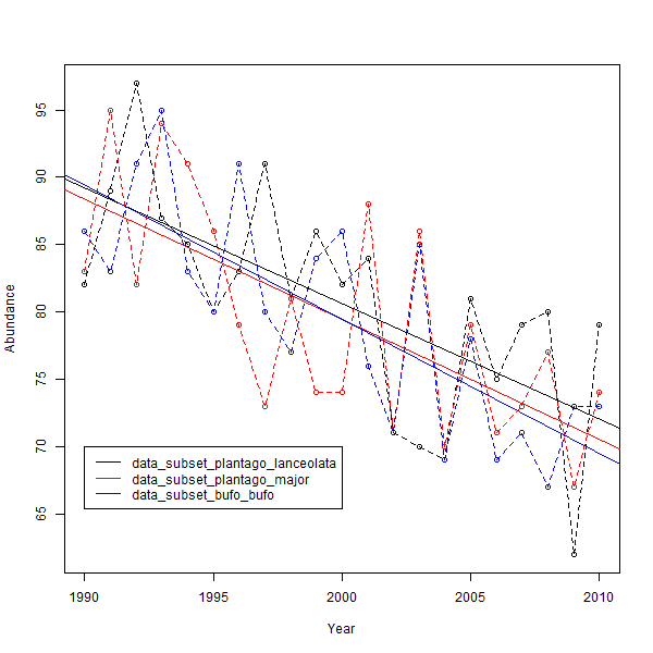
plot_combined <- function(models,data_subsets){
  file_name <- "plot_combined.png"
  png(file=file_name,width=600, height=600)
  
  #add the datasets
  plot(data_subsets[[1]]$time,data_subsets[[1]]$abundance,xlab = "Year",ylab="Abundance")
  points(data_subsets[[2]]$time,data_subsets[[2]]$abundance,col = "red")
  points(data_subsets[[3]]$time,data_subsets[[3]]$abundance,col = "blue")
  
  #join the dots
  lines(data_subsets[[1]]$time,data_subsets[[1]]$abundance,lty=2)
  lines(data_subsets[[2]]$time,data_subsets[[2]]$abundance,col = "red",lty=2)
  lines(data_subsets[[3]]$time,data_subsets[[3]]$abundance,col = "blue",lty=2)
  
  #add the lines from the models
  abline(models[[1]])
  abline(models[[2]],col = "red")
  abline(models[[3]],col = "blue")
  
  #add a legend
  legend(1990, 70, legend=names(data_subsets)[1:3],
         col=c("black","red", "blue"),lty=1)
  
  dev.off()
  
  #return just the file name
  file_name
  
}


### targets workflow

#first we need to define sub workflows split into data files for each species
mapped <- tar_map(
  #map over the interested species dataframe
  values = interested_species,
  
  #each thing we do for all species
  tar_target(data_subset, subset_data(data,foc_species)), #subset to only that species
  tar_target(subset_model, fit_model(data_subset)), #fit a model
  tar_target(out_plot,plot_with_line(data_subset,subset_model,foc_species)) # make a plot
)

#built the workflow list
list(
  tar_target(data_file, "abundance.csv",format="file"),
  tar_target(data ,read.csv(data_file)),
  
  # sub workflow defined above for each species
  mapped,
  
  #first combine them to lists of each data type simply using the list() function
  tar_combine(models_list,mapped$subset_model,command = list(!!!.x)),
  tar_combine(data_list,mapped$data_subset,command = list(!!!.x)),
  
  #then make a plot using the normal tar_target functions using the combined targets
  tar_target(combined_plot,plot_combined(models_list,data_list),format = "file")

)

Final plot should look something like this

tar_visnetwork()