Notes from ESHG Göteborg 2019
PL1.1 Ulrike Peters: Genetic epidemiology of colorectal cancer - from discovery to prevention
C09.1: Noah Zaitlen: Germline genetic variation drives the somatic landscape of tumors
-
not the main one: Extremely low-coverage sequencing and imputation increases power for genome-wide association studies (Pasanuic et al. 2012 Nat Genet)
-
human is the environment of the tumor
-
relationship between germline + somatic mutations
- n=100K with sequenced cancer genome
- low X sequencing
- SBT (seeing beyond the target): examine off-target reads in (software stitch for low X): imputation of low X reads.
- correlation between genetic ancestry and germline genotypes is high
- long tail of somatic mutations
- smoking signature
- smoking signature differs between ancestries
- more with PCA genetics ancestry

PRS for smoking + total mutational burden (?)
Models for germline
- germine gt > exposure > distal somatic mutations (heritable exposure)
- germline gt alters the somatic mutation > leads to local and distal somatic mutations


C11.1: Zoltán Kutalik: Maximum likelihood method quantifies the overall contribution of gene-environment interaction to complex traits: an application to obesity traits
- Maximum likelihood method quantifies the overall contribution of gene-environment interaction to continuous traits: an application to complex traits in the UK Biobank (Sulc et al. 2019)
C11.2: Ninon Mounier: Leveraging correlated risks to increase power in Genome-Wide Association Studies
- Genomics of 1 million parent lifespans implicates novel pathways and common diseases and distinguishes survival chances (Timmers, Mounier et al. 2019)
C11.3: Hieab H. Adams: One and a half million genome-wide association studies of brain morphometry: a proof-of-concept study

About: Genetics of brain structure
By: ENIGMA, cohorts for heart and aging research in genomic epidemiology
- Full exploitation of high dimensionality in brain imaging: The JPND working group statement and findings (Adams et al. 2019)
- Partial derivatives meta-analysis: pooled analyses when individual participant data cannot be shared (Adams et al. 2016)
- Heritability of the shape of subcortical brain structures in the general population (Roshchupkin et al. 2016)
- what is the total size of the brain (GWAS done): crude measure - similar to only studying genome with karyogram
- subcortical structure - similar to FISH
- cortical brain region - similar to array CGH
- shape of subcortical structures, results in 54K variables: shape heritable - similar to WES
- voxel-based morphometry (similar to WGS), 1.5 mio variables
- n=18K, middle age and elderly
- European ancestry
- used for proof of concept
- amount of computation time
- data transfer
- multiple testing correction (trillion of tests)
- novel approach of meta-analysis (partial derivative meta analysis, see adams et al. biorxiv)
- running software for running large GWAS (HASE software)
- for genotypes: MAF > 0.05, R2 > 0.3
- for brain images: removing low density voxel
- genome: large number of SNPs
- brain: 62K unique voxels, 55 brain regions
C11.4: Maarja Lepamets: Genome-wide copy number variant association study reveals several novel disease-associated loci
About: CNV studies
- genotyping arrays for CNVs are not ideal, can only capture CNV values between 0 and 4
- CNV detection done with pennCNV
- WGS from 983 Estonians
- half (0.4) of the CNVs are missing (FN)
- 0.008 probability of FP
Previous method by Aurelien Mace

- CNV quality evaluation with gene expression (GE) and methylation data (MET).
- mix of three score: WGS score, MET score and GE Score
- harmonise CNVs (various lengths and breakpoints)
- only del, only dup, only minor effects
Phenotypes
- T2D
- IBD: previous score did not work
- CD: new hits
C11.5: Ross Byrne: Population structure and demographic change
- n = 1626 dutch samples (from an ALS study)
- ~ 300K SNPs overlap
- geolocation
- pop structure = existince of subgroups in an super populations
use of chromosome painting to avoid removing SNPs in LD
- finds local population structure (PC1 and PC2) - not working with normal PCA on SNPs
- regional ancestry with German (north influence), French, Belgium (south influence), Danish
- lower diversity of the north (split south-north in 600 AD)
- looking at the length of haplotypes: short haplotypes = older. then doing PCA on these binned clusters

C11.6: Marie Verbanck: The landscape of pervasive horizontal pleiotropy in human genetic variation is driven by extreme polygenicity of human traits and diseases
- The landscape of pervasive horizontal pleiotropy in human genetic variation is driven by extreme polygenicity of human traits and diseases (Jordan, Verbanck & Do 2019)
- Detection of widespread horizontal pleiotropy in causal relationships inferred from Mendelian randomization between complex traits and diseases (Verbanck et al. 2018)
Definition: single genetic element having multiple distinct phenotypic effects
Two types
- vertical pleiotropy: leveraged in causal inference
- biological (single-locus) horizontal pleiotropy: not well measured today
- using a collection of summary statistics
- define for each phenotypes a vector of z scores, normalise them to be N(0,1)
- whitening procedure to remove dependence between traits
Two types of pleiotropic score
- total magnitude of the effect the variant has (Pm, m for magnitude)
- number of traits pleiotropy score (Pn)
SNV1 in LD with SNV2. SNV1 has an effect of T1, SNV2 has an effect on T2.
- therefore regress out the effect of LD scores from the pleiotropy score
- additionally take polygenicity into account
- UKBB
- only heritable phenotypes (p=372)
Enrichment analysis:
- more pleiotropy in UTR, Promotor, Transcription and regulation and enhancer
- less in quiescent/ heterochromatin
- more pleiotropy in eqtls
- GWPS (GWAS with Pm and Pn as outcome)


Also: Marie Verbanck is moving to a new position in Paris.
- manual curation and ML methods
- the basis of the catalog are GWAS publications
- surprised to see that as criterium, only GWAS from array data (?)
S07.1: Krista Fischer: Polygenic risk scores in genetic epidemiology
- Polygenic prediction of breast cancer: comparison of genetic predictors and implications for risk stratification (Läll et al 2019, BMC Cancer)
- history of GRS, emerged around 2012
- weighted sum of SNP effects
- what is the optimal selection of SNPs: not only significant
How to build a PGRS?
- Use a large GWAS (how to choose? large sample size, ancestry?)
- How to handle LD? (either LD pruned/clumped SNPs OR use method that accounts for LD structure)
Winner's curse: relationship between estimated effect size and p-value (smaller p-value the more effect size is overestimated)
Solution: use extra weight to account for this winners curse: doubly weighted score.
They looked at the incident T2D: analysis of 638 incident cases in overweight (but not obese).
Läll et al 2019, BMC Cancer: different companies would report different risks.
- combine m PGRSs scores
- works similarly like doubly-weighted approach
- LDpred: would it work better?
- Lasso regression? may work slightly better
- Disease-free baseline survival
- Effect of non-genetic risk factors
- Effect of PGRS?
Implemented in Estonian biobank: genetic risk prediction and environment prediction (e.g. CVD GRS prediction, and depending on BMI).
- not a diagnostic tool, but a predictive tool
- Khera et al. 2018
- no best methodology
- PGRS is not unique (depends on GWAS used)
- PGRS is ancestry-specific
- moving towards personalised risk prediction
S07.2: Samuli Ripatti: Polygenic risks and their impact on behavior
- Presents two parts
- Finriski calculator
- kardioKompassi
- Framingham risk score vs 13 SNPs (2010) and 6.4 m SNPs
- what has changed? better input with larger GWAS, better algorithms and better tests sets (UKBB)
- A multilocus genetic risk score for coronary heart disease: case-control and prospective cohort analyses (Ripatti et al. 2010)
- From genetic discovery to future personalized health research (Palotie, Widén & Ripatti 2013)
- Geographic Variation and Bias in the Polygenic Scores of Complex Diseases and Traits in Finland (Kerminen et al. 2019)
- 500K = 10% of the population
- combination of existing cohorts + new biobanking efforts
- past 50 years phenotypic data of registry
- Summary stats + LD panel
- T2D: 17K cases
- Prostate Cancer
- Prostate Cancer Death
- e.g. effect of certain mutations, frameshift mutation
- Does it matter to communicate back the risk based on a few weak effects SNPs? Nope, not really
- But genetic information based on a few strong effect SNPs (BRCA) does.
- What about GRS in Finland? GeneRISK
- n ~ 7000
- some at high risk for CVD
- kardioKompassi

- 40% were at high risk previously
- follow-up after 1.5 years
- 15% stopped smoking
- 16% started losing weight
- females change a lot
Done by Elisabeth Widen.
Good PRGS + communicative tools = change in behaviour
S07.3: Rosalind Eeles: Polygenic risk scores in prostate cancer
- Association analyses of more than 140,000 men identify 63 new prostate cancer susceptibility loci (Schuhmacher et al. 2018)
- prostate cancer prevalent and underdiagnosed in Africa
- prostate cancer is 50% more common in identical twins than non-identical ones
- what contributes to risk: rare (small effect size) and common variants (large effect size)
- game-on consortium and practical consortium
- onco array
- n > 100K
- 27 of the loci were associated with aggressive and early-onset prostate cancer
S10.1: Christian Benner: From association to causal variant(s): statistical methods for finemapping
- FINEMAP: efficient variable selection using summary data from genome-wide association studies (Benner et al. 2016)
- FINEMAP tool
- PON1 gene with PON1 enzymatic activity in finrisk
- Genomic regions can harbour many genetic variants
- Summary statistics fine-mapping
- Uses shotgun stochastic search (Hans et al. 2007)
y = x beta + eps(xgenotype,betaeffect size,yphenotype)- vary
xas the genotypes (singletons, pairs, triplets, ...) - using bayes factor that uses summary level data
- speeding up search with shotgun search (similar to MCMC)
- LIPC association with HDL cholesterol (Surakka et al. 2015): pinpointing to 3 other variants than when doing conditional analysis.
- PON1 gene with PON1 enzymatic activity in finrisk: difficult to pinpoint variants
- Uses only summary stats
- scales to large genomic regions
- Ex: APOE association with LDL cholesterol: 3 variants found with GWAS manual fine mapping + FINEMAP
- if 1KG-FIN was used to calc LD, then other variants are found
- simulation with NFBC and FINRISK: NFBC used for summary statistics + LD and FINRISK only for LD
- Relationship between GWAS size and LD panel size: misspecified LD can cause FP and FN
- hypothesis: large part of heritability could be explained by the fine-mapped variants
- motivation: PON1. 5 lead variants explain 70%, bolt explains a bit less.
- setting: BOLT vs FINEMAP
- when small effects: FINEMAP underestimates
- when large effects: FINEMAP has smaller MSE
- Utility of FINEMAP heritability?
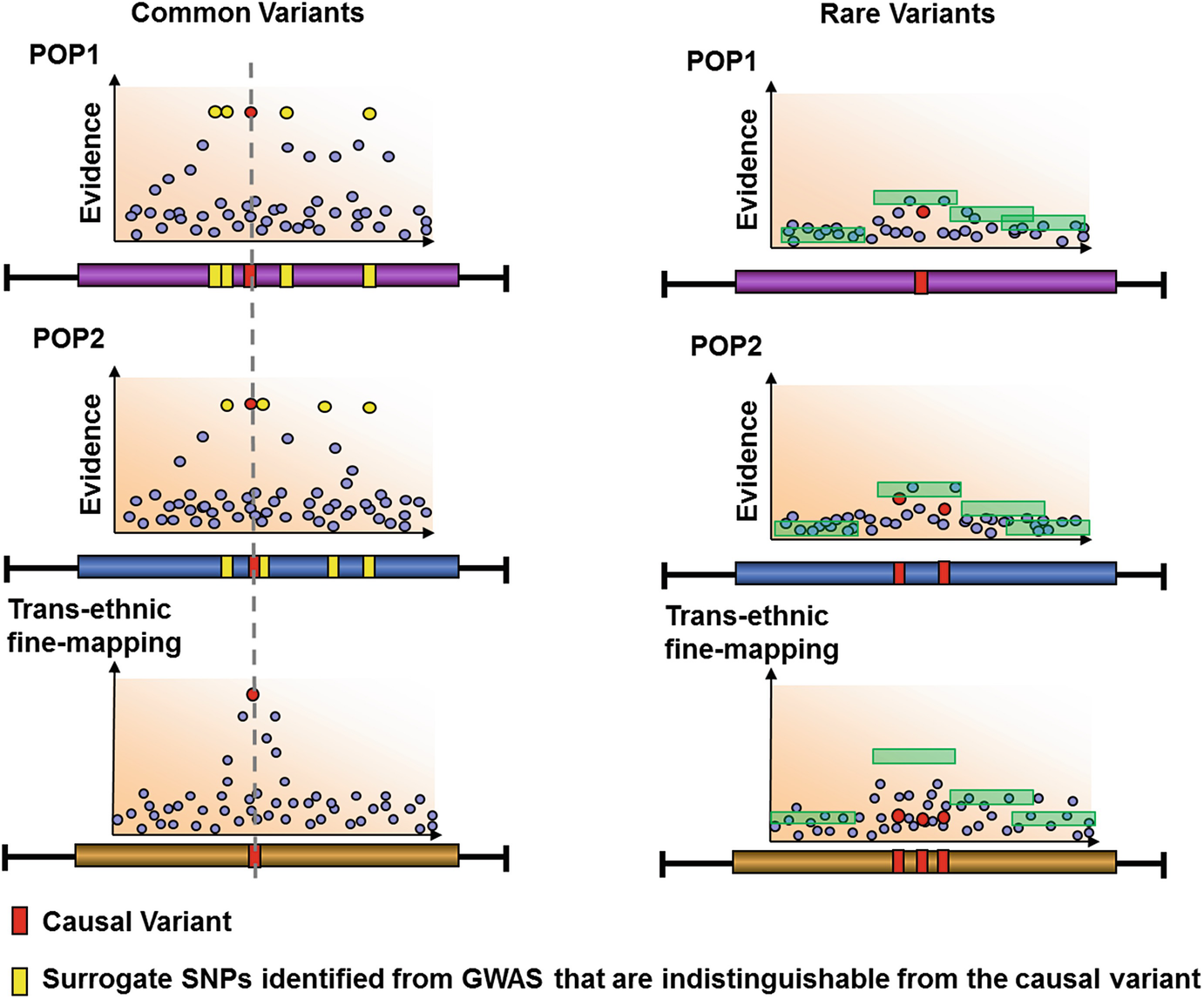
S10.2: Andrew P. Morris: Leveraging genome-wide association studies in diverse populations to fine-map complex human trait loci
- Trans-ethnic meta-regression of genome-wide association studies accounting for ancestry increases power for discovery and improves fine-mapping resolution (Mägi et al. 2017)
- Genome-wide trans-ancestry meta-analysis provides insight into the genetic architecture of type 2 diabetes susceptibility (DIAGRAM Consortium et al. 2014)
- Transethnic meta-analysis of genomewide association studies (Morris 2011)
- LD: enables efficient efficient discovery of complex traits through GWAS array design + imputation
- LD: hinders fine-mapping, because similar/exchangeable association
- Extent of LD is weakest in African ancestry populations: hence optimal for fine-mapping
- Trans-ethnic fine-mapping includes summary statistics from diverse populations

Genomewise trans-ancestry meta-analysis provides insight into the genetic architecture of type2 diabetes susceptibility gives evidence to a model that the underlying causal variants are shared across global populations and arose prior to human pop migration out of Africa. Argues against "synthetic association" hypothesis.
- Benefits in modelling heterogeneity that is correlated with differences between populations

- Article: Morris 2011
- Similar to a Bayesian partition model
- Uses summary statistics
- Takes account of the expected similarity in allelic effects between the most closely related populations, while allowing for heterogeneity between more diverse ethnic groups
- n=22K cases + 40Kcontrols
- from EUR, SAS, EAS, Hispanic, African American ancestry groups
- first step: on basis of pair-wise mean allele frequency differences across the five loci: three clusters (Asian vs American vs European)
- Article: Mägi et al. 2017
- projects studies onto axes of genetic variation
- includes principle components as covariates

S10.3: Sara L. Pulit: Large scale integration of genetic and -omics data to find susceptibility genes for obesity and fat distribution
- Meta-analysis of genome-wide association studies for body fat distribution in 694 649 individuals of European ancestry (Pulit et al. 2019)
- Github repo
- Difference between obesity (measured with BMI) vs. fat distribution (measured with WHR adjusted for BMI)
- WHR adj: pear vs apple shaped (decreased vs increased risk for metabolic syndrome/T2D)
- UKB LMM BOLT + meta-analysis with GIANT: > 300 signal
- WHR is genetically sex dimorphic: genetics effect tend to be stronger in women than men
- next: check enrichment of GWAS signals in human tissue: FUMA
- WHR not associated with Brain Tissue
- obesity (BMI) not associated with brain tissue
- next: fine-mapping


- separate between GIANT vs UKBB
- 1st problem: difference in number of SNPs: 2.5 M vs 27 M analyse separately, using GIANT as replication
- 2nd problem: GIANT compromised between sub-cohorts, LD not accessible vs. UKB homogeneous and LD accessible

- finds enrichment of likely causal EZH2 binding sides
- fine-mapping and enrichment testing reveals sex-specific effects (potential role for EZH2)
- what phenotype results from perturbing EZH2?
C16.4: Nina J. Mars: High polygenic risk contributes to an early disease onset in common cardiometabolic diseases and cancers
C21.5: Hanieh Yaghootkar: Genome-wide association study of MRI liver iron content in 9,800 individuals yields new insights into its link with hepatic and extrahepatic diseases

S16.1: Hilary Finucane: Leveraging polygenic signals for insight into disease biology
- Heritability enrichment of specifically expressed genes identifies disease-relevant tissues and cell types (Finucane et al 2018 Nat Genet)
- Interrogation of human hematopoiesis at single-cell and single-variant resolution (Ulirsch et al 2018 Nat Genet)
Ways to prioritize genes at a locus:
- fine-map coding variant?
- use eQTLs (e.g. EWAS, eCaviar)
- local functional genomics
- closest gene
- similarity/network closeness
- Leveraging genome-wide enrichment: what about patterns that are constant across phenotypes (e.g. similar GEXPR enrichment patterns in BMI and schizophrenia)
- n Gene by p Gene features
- vector with (likely disease gene) and (less likely disease gene)
- predict "how likely a disease gene" is from a new gene data features
MAGMA model
- LOCO approach
- pvalue
Input:
- Summary stats
- LD panel
- Gene feature matrix
Output:
- gene scores and p-values
- With gold standard genes: not lots of gold standard
- "Benchmarker" for polygenic signal: Fine et al 2019 AJHG
- how to quantify confidence?
- can we estimate P(causal|prioritised & in locus)? see Stacey et al 2019 nucleic acids reserach
- for 30-70% of loci, closest gene = causal gene
- vs. P(causal | prioritised & closest)
Top features
- Mouse and GO terms
- ACE gene
- FCER1G gene
S16.2: George Davey-Smith: Genetic instruments in mendelian randomization studies
- Within-family studies for Mendelian randomization: avoiding dynastic, assortative mating, and population stratification biases (Brumpton et al 2019)
S16.3: Manuel Rivas: Large-scale inference of human genetic data
https://biobankengine.stanford.edu/
S18.3: Alicia Martin: Consequences of population genetic differences in genetic risk prediction across diverse human populations
- Population histories of the United States revealed through fine-scale migration and haplotype analysis (Dai et al. 2019)
- Polygenic adaptation on height is overestimated due to uncorrected stratification in genome-wide association studies (Sohail et al. 2019)
- Human Demographic History Impacts Genetic Risk Prediction across Diverse Populations (Martin et al. 2017)
- Genetics has a huge diversity problem 70% European
- How do biases in genetics impact the generalisability of knowledge with respect to different populations?
- Causal variant effects are mostly shared across populations
- AF, LD, environment and other factors differ?
- Dai et al. 2019 and Martin et al. 2017
- Polygenic scores differs, but biases are not meaningful
- neutral evolution is sufficient to explain biases
- See Sohail et al. 2019
- using UKB for polygenic score better than GIANT
- Also affects local population: FINRISK
- See Geographic Variation and Bias in the Polygenic Scores of Complex Diseases and Traits in Finland (Kerminen et al. 2019)
- UKBB works best, not FINRISK or GIANT PRS

In UKBB
- Europeans are best predicted,
- American 1.6 less
- SAN
- African 4.5 x less
GWAS is best powered to discover common variants in the population we are studying
- LD differences across populations
- Biology and causal variants mostly shared, but estimations differ
- Environment, selection, and other complicated differences (e.g. heritability differences)

- Ancestry matches or not
- If discovery is UKBB, then the prediction in BBJ is less good. But when BBJ is uses, then UKBB prediction is almost equally good (differences in BBJ)


EUR 3x larger sample size than EAS (13K cases)
- 35K Africans (AS, Kenya, Uganda, Ethiopia), to study genetic risk of schizophrenia
- HRC: 32K reference panel,
- Capacity building: in-depth training program (GINGER), see Advancing neuropsychiatric genetics training and collaboration in Africa (van der Merwe et al. 2018)
- Neuropsychiatric Genetics of African Populations-Psychosis (NeuroGAP-Psychosis): a case-control study protocol and GWAS in Ethiopia, Kenya, South Africa and Uganda (Stevenson et al. 2018)

- GWASs from three populations
- approach: consider cross population to calibrate effect sizes in each pop
- related methods: LD score and MTAG

- PRS increase disparities due to Eurocentric GWAS biases
- more diverse GWAS studies and new methods
- communicate culturally sensitive topics responsibly and wildly
C25.1: Tom G. Richardson: A transcriptome-wide Mendelian randomization study to uncover tissue-dependent regulatory mechanisms across the human phenome
- A transcriptome-wide Mendelian randomization study to uncover tissue-dependent regulatory mechanisms across the human phenome (Richardson et al. 2019)
- mrcieu.mrsoftware.org/Tissue_MR_atlas
Multivariate GWAS of inflammatory markers reveals novel disease associations
-
each variant with multiple phenotypes are tested
-
apply multivariate GWAS + find out which traits and SNPs were driving the associations
-
multivariate GWAS: MetaCCA (Cichonska et al. 2016)
-
CCA does not output effect size and se, hence no FINEMAP
-
solved by decomposing the multivariate GWAS results again on a single variant level.
-
MetaPhat (Lin et al. 2019): tool to detect and decompose multivariate associations from univariate GWAS stats.

C25.6: Tzung-Chien Hsieh: GestaltMatcher: Identifying the second patient of its kind in the phenotype space
- How to identify another patient with a rare phenotype?
- This is important to increase power for analysis
- Using facial representation
- matching patient to other people in a database
- Data used: PEDIA
- extract facial features, deep convolutional network


Nordin et al. 2019 https://www.biorxiv.org/content/10.1101/660241v1