Created
April 16, 2018 09:43
-
-
Save tuner/608801362befe42577f4666671bc965c to your computer and use it in GitHub Desktop.
Stochastic neighborhood embedding in R
This file contains bidirectional Unicode text that may be interpreted or compiled differently than what appears below. To review, open the file in an editor that reveals hidden Unicode characters.
Learn more about bidirectional Unicode characters
| # | |
| # (c) Kari Lavikka 2018 | |
| # | |
| library(stats) | |
| source("mnist.R") | |
| mnist <- load_mnist() | |
| sample_and_reduce_mnist <- function(n, dimensions = 50) { | |
| sampled_indexes <- sample(train$n, n) | |
| classes <- train$y[sampled_indexes] | |
| mnist_subset <- train$x[sampled_indexes, ] | |
| mnist_subset <- mnist_subset[, colSums(mnist_subset) != 0] | |
| mnist_pca <- prcomp(mnist_subset, center = T, scale. = T) | |
| list( | |
| digits = mnist_pca$x[, 1:dimensions], | |
| classes = classes | |
| ) | |
| } | |
| reduced <- sample_and_reduce_mnist(1000, 50) | |
| x <- reduced$digits | |
| pairwise_distance <- function(x, i, j) ifelse(i == j, Inf, sum((x[i, ] - x[j, ])^2)) | |
| compute_probabilities <- function(x, perplexity) { | |
| p <- 1 / (2 * perplexity^2) | |
| t(sapply(seq_len(nrow(x)), | |
| function(i) { | |
| dk <- sapply(seq_len(nrow(x)), | |
| function(j) exp(-pairwise_distance(x, i, j) * p)) | |
| dk / sum(dk) | |
| })) | |
| } | |
| # Q = probabilities in induced space | |
| # P = probabilities in original space | |
| compute_loss <- function(Q) sum(ifelse(Q > 0, P * log(P / Q), 0)) | |
| # y = values in induced space | |
| compute_gradient <- function(y, Q) { | |
| n_seq <- seq_len(nrow(y)) | |
| t(sapply(n_seq, | |
| function(i) | |
| 2 * rowSums(sapply(n_seq, | |
| function(j) (y[i, ] - y[j, ]) * (P[i, j] - Q[i, j] + P[j, i] - Q[j, i])) | |
| ))) | |
| } | |
| # y = values in induced space | |
| gradient_descent <- function(y, step_function) { | |
| loss <- Inf | |
| min_loss <- Inf | |
| iters_since_last_min <- 0 | |
| rounds <- 0 | |
| best_y_so_far <- numeric() | |
| losses <- numeric() | |
| alphas <- numeric() | |
| while (iters_since_last_min < 20 & rounds < 600) { | |
| Q <- compute_probabilities(y, 0.5) | |
| gradient <- compute_gradient(y, Q) | |
| alpha <- step_function(loss) | |
| alphas <- c(alphas, alpha) | |
| y <- y - alpha * gradient | |
| loss <- compute_loss(Q) | |
| losses <- c(losses, loss) | |
| if (loss < min_loss) { | |
| min_loss <- loss | |
| iters_since_last_min <- 0 | |
| best_y_so_far <- y | |
| } else { | |
| iters_since_last_min <- iters_since_last_min + 1 | |
| } | |
| rounds <- rounds + 1 | |
| message("Round: ", rounds) | |
| message("Loss: ", loss) | |
| plot(y[, 1], y[, 2], col = reduced$classes + 1, pch = 19, cex = 0.7) | |
| title(paste("Loss =", loss)) | |
| } | |
| list( | |
| y = best_y_so_far, | |
| losses = losses, | |
| alphas = alphas | |
| ) | |
| } | |
| create_adaptive_schedule <- function(acceleration, penalty) { | |
| step_size <- 0.5 | |
| previous_loss <- Inf | |
| function(loss) { | |
| step_size <<- step_size * ifelse(loss < previous_loss, acceleration, penalty) | |
| previous_loss <<- loss | |
| step_size | |
| } | |
| } | |
| P <- compute_probabilities(reduced$digits, 3.5) | |
| # Begin with randomized y | |
| y <- matrix(rnorm(nrow(x) * 2, 0, 0.1), ncol = 2) | |
| results <- gradient_descent(y, create_adaptive_schedule(1.02, 0.5)) | |
| # Plot the result | |
| with(results, plot(x[, 1], x[, 2], col=reduced$classes + 1, pch = 19, cex = 0.7)) | |
| # Testing with t-SNE | |
| library(Rtsne) | |
| tsne_result_30 <- Rtsne(x, perplexity = 30, pca = F, verbose = T) | |
| plot(tsne_result_30$Y, col = reduced$classes + 1, pch = 19, cex = 0.8) | |
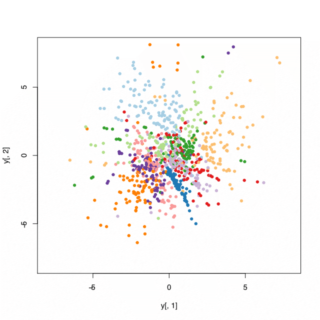
And here is an example output from the script:
Sign up for free
to join this conversation on GitHub.
Already have an account?
Sign in to comment
https://gist.github.com/brendano/39760 .. here's the script that loads the mnist data