MGN.md

Multi-scale Gaussian Normalization

---

I have already mentioned the differences between Cadair's and Eric's implementation in this comment. Please note the differences mentioned for Eric's implementation are actually not present. Eric has confirmed it here. When I read through Eric's implementation it became clear that Eric's code is actually following the paper exactly. As far as Cadair's code is comnsidered it has some differences, which I rectified. Now both the implementation follow the paper. But there were still differences which could be spotted.

Rectified Cadair's code

if weights is None:
        weights = np.ones(len(sigma))

    # 1. Replace spurious negative pixels with zero
    data[data <= 0] = 1e-15  # Makes sure that all values are above zero
    image = np.empty(data.shape, dtype=data.dtype)
    conv = np.empty(data.shape, dtype=data.dtype)
    sigmaw = np.empty(data.shape, dtype=data.dtype)

    for s, weight in zip(sigma, weights):
        # 2 & 3 Create kernel and convolve with image
        ndimage.filters.gaussian_filter(data, sigma=s,
                                        truncate=truncate, mode='nearest', output=conv)
        # 5. Calculate difference between image and the local mean image,
        # square the difference, and convolve with kernel. Square-root the
        # resulting image to give ‘local standard deviation’ image sigmaw
        conv = data - conv
        ndimage.filters.gaussian_filter(conv ** 2, sigma=s,
                                        truncate=truncate, mode='nearest', output=sigmaw)
        np.sqrt(sigmaw, out=sigmaw)
        conv /= sigmaw

        # 6. Apply arctan transformation on Ci to give C'i
        conv *= k
        np.arctan(conv, out=conv)
        conv *= weight

        image += conv

    # delete these arrays here as it reduces the total memory consumption when
    # we create the Cprime_g temp array below.
    del conv
    del sigmaw

    # 8. Take weighted mean of C'i to give a weighted mean locally normalised
    # image.
    image /= len(sigma)

    # 9. Calculate global gamma-transformed image C'g
    data_min = data.min()
    data_max = data.max()
    Cprime_g = (data - data_min)
    Cprime_g /= (data_max - data_min)
    Cprime_g **= (1/gamma)
    Cprime_g *= h

    image *= (1 - h)
    image += Cprime_g

    return image

There were no changes made to Eric's code.

---

Visual differences

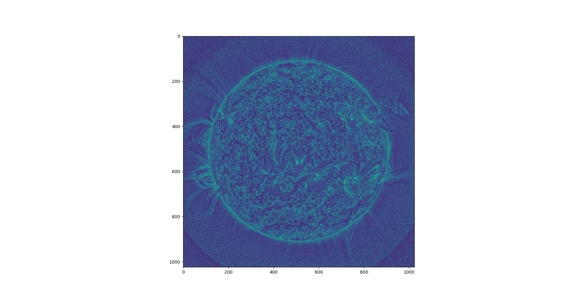
Raw Matplotlib Output

Cadair's Output

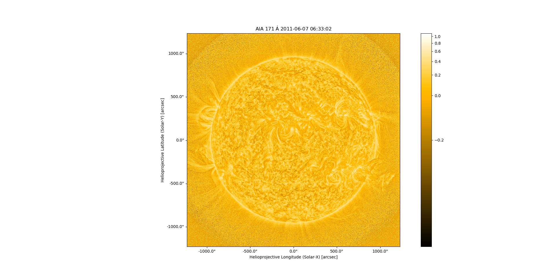
Eric's Output Sunpy Map Output

Cadair's Output

Eric's Output

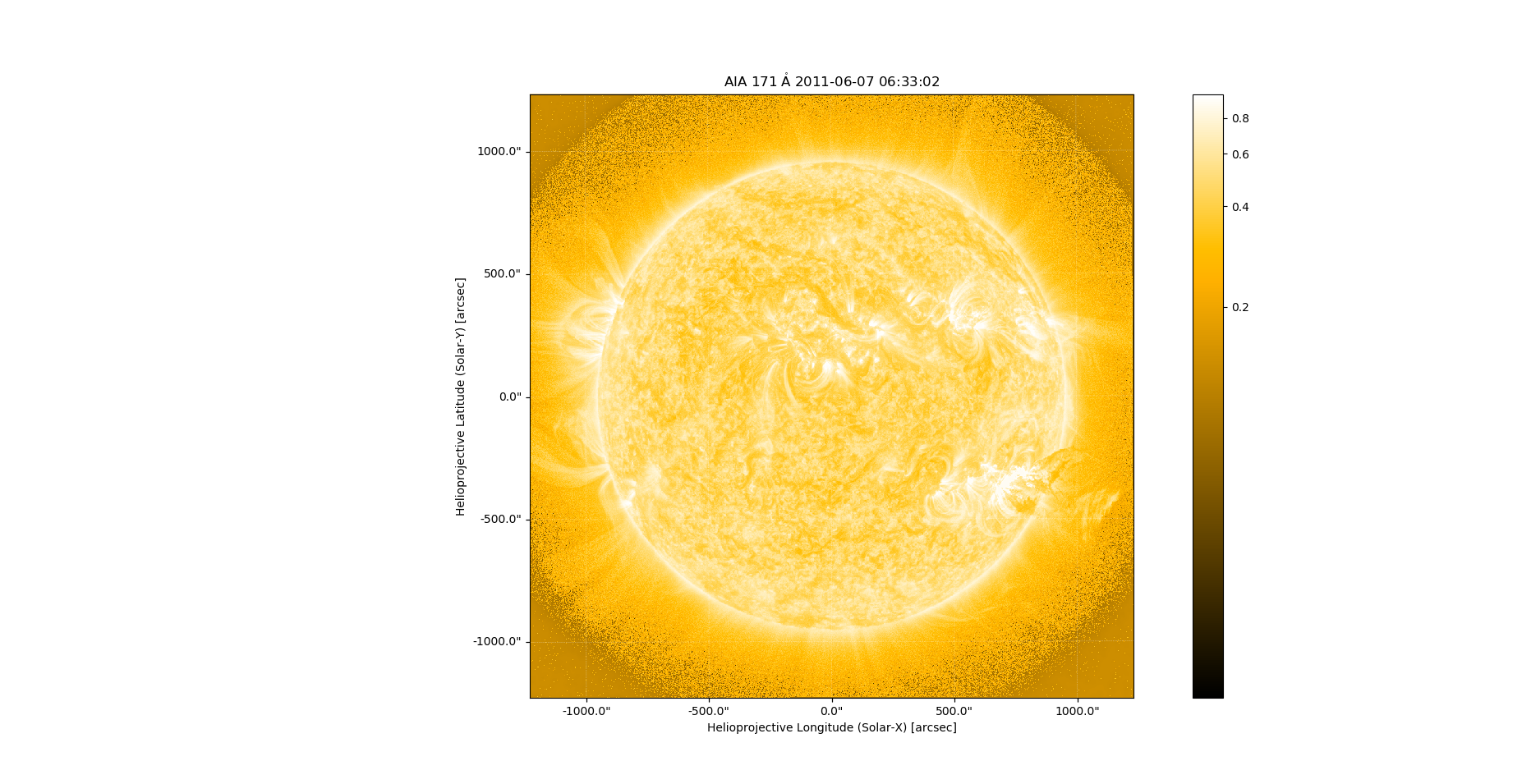
By visual inspection, it is clear that both the implementation are giving more or less the same result. Though it should be noted that the rectified Cadair's implementation show the structures in greater detail as the contrast is much better. Both the implementation are very similar and outputs too.