
Pic credits : Github
Welcome back peeps. We are now starting System Design Series ( over weekends) where we will cover how to design large ( and great) systems, the techniques, tip/tricks that you can refer to in order to scale these systems. As a senior software engineer it’s expected that you know not just the breadth but also depth of the system design concepts.
2. Horizontal and vertical scaling
3. Load balancing and Message queues
6. Networking, How Browsers work, Content Network Delivery ( CDN)
7. Database Sharding, CAP Theorem, Database schema Design
8. Concurrency, API, Components + OOP + Abstraction
9. Estimation and Planning, Performance
In layman’s language, system design is about —
Architecture + Data + Applications
Architecture means how are you going to put the different functioning blocks of a system together and make them seamlessly work with each other after taking into account all the nodal points where a sub-system can fail/stop working.
One such architecture example is shown below —
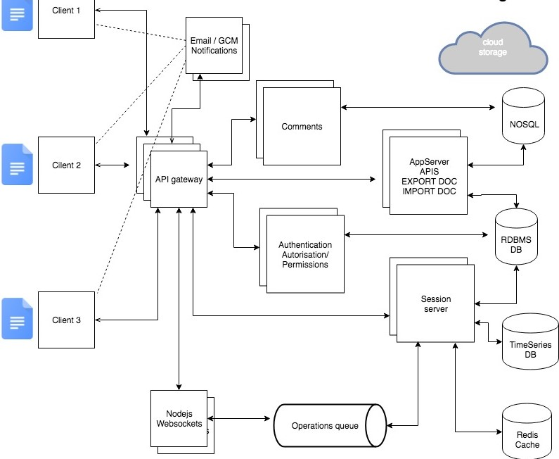
Pic credits : twtr
Data means what is the input, what are the data processing blocks, how to store petabytes of data and most importantly how to process it and give the desired/required output.
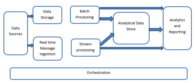
Pic credits : researchgate
Applications means once the data is processed and output is ready how are the different applications attached to that large back end system will utilize that data.
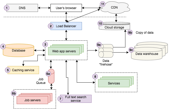
Pic credits : ResearchGate
All this is prepared in the form of a large pipeline ( some/most part of it is automated based on the requirements)
Again, designing larger system that can serve zillions of people have 4 things in common —
- Reliability : It’s measured in terms of robustness, failures and effect analysis of the sub systems of the larger system.
- Scalability : It’s measured in terms of resources allocation, utilization, serviceability and availability.
- Availability : It’s measured by the percentage of time in a given period that a system is available to perform the assigned task without any failure(s).
- Efficiency : It’s measured in terms of reusability of components, simplicity and productivity.
And all of it bottles down to three things — Cost, Speed and Failures.
Now let’s talk about the most important concepts ( technically you should know) in System Design
2. Proxies
3. Caching
4. CAP theorem
6. Replication
7. Sharding and Data Partitioning
10. Storage, Availability and Hashing
11. API
- Horizontal and vertical scaling: Imagine you have a toy shop and you have a limited number of toys. If you want to make room for more toys, you can either stack them up vertically (vertical scaling) or you can spread them out horizontally (horizontal scaling). The same goes for computer systems, if you want to make it work faster, you can either add more power to it (vertical scaling) or you can add more computers to it (horizontal scaling).
- Load balancing and Message queues: Imagine you have a bunch of friends who want to play a game together, but you only have one game. To make it fair, you take turns playing the game. This is like load balancing in a computer system, it makes sure that the work is evenly distributed so it runs smoothly. Message queues are like a line or queue where you and your friends wait for your turn to play the game. In a computer system, message queues are used to store messages or tasks until they can be processed.
- High level design and low level design: Imagine you and your friends want to build a treehouse. The high level design is like the big picture plan of what the treehouse will look like and what it will have. The low level design is like the details of how each part of the treehouse will be built. The same goes for computer systems, the high level design is the big picture plan, and the low level design is the details of how it will be built.
- Consistent Hashing, Monolithic and Microservices architecture: Imagine you have a toy box and you want to keep all your toys organized. You can either keep all your toys in one big box (monolithic) or you can keep them in many small boxes (microservices). Consistent hashing is like labeling each box so you know what toys are in it. In a computer system, consistent hashing helps with organizing data in a distributed system.
- Caching, Indexing, Proxies: Imagine you have a big library with many books. To find a book quickly, you can either make a list of all the books (indexing) or you can keep a copy of the book you often look for in a nearby shelf (caching). A proxy is like a helper who can get the book for you if you can’t find it. In a computer system, caching, indexing and proxies are ways to make information easier to find and faster to access.
- Networking, How Browsers work, Content Network Delivery (CDN): Imagine you want to send a message to your friend who lives far away. To send the message, you can either go to your friend’s house (not efficient) or you can send the message through a network of people (more efficient). Browsers are like a messenger who helps you find websites on the internet and CDN is like a big network of messengers who can deliver the website to you faster.
- Database Sharding, CAP Theorem, Database schema Design: Imagine you have a big notebook with many pages and you want to keep your notes organized. You can either keep all your notes in one big notebook (not efficient) or you can divide your notes into many small notebooks (database sharding). The CAP theorem is like a rule that helps you decide what kind of notebook you want to use. The database schema design is like how you want to organize your notes in each notebook.
- Concurrency, API, Components + OOP + Abstraction: Imagine you and your friends want to play a game together. You can either play the game one by one (not efficient) or you can play the game at the same.
- Networks & Protocols: Imagine you and your friends want to send secret messages to each other. To make sure the messages are safe, you can use a secret code (protocol) and send the messages through a network of friends (network). In a computer system, networks and protocols are used to send information safely and efficiently.
- Latency & Throughput: Imagine you and your friends are playing a game where you have to pass a ball to each other as fast as you can. Latency is like the time it takes for the ball to get from one friend to another, and throughput is like how many balls can be passed in a certain amount of time. In a computer system, latency and throughput are important for measuring the speed and efficiency of information transfer.
- Storage, Availability, and Hashing: Imagine you have a toy box and you want to keep your toys safe and organized. To keep your toys safe, you can lock the toy box (storage) and make sure it’s always available to you (availability). To keep your toys organized, you can label each toy with a special code (hashing). In a computer system, storage, availability, and hashing are important for keeping information safe and organized.
- Start with requirements: Clearly understand the requirements and constraints of the system before starting the design process.
- Scalability: Design the system with scalability in mind from the beginning to ensure it can handle increasing workloads over time.
- Modularity: Design the system as a set of modular components that can be developed, tested, and maintained independently.
- Abstraction: Use abstraction to separate the implementation details from the interfaces, making the system easier to understand and maintain.
- Performance: Consider performance trade-offs when making design decisions, such as using caching or load balancing to improve response time.
- Availability: Design the system for high availability by using redundancy and failover mechanisms, such as load balancers or database replication.
- Security: Consider security risks and implement appropriate security measures, such as encryption, authentication, and authorization.
- Monitoring: Implement monitoring and logging to keep track of system performance and detect and diagnose issues.
- Testability: Design the system for testability, including unit tests, integration tests, and end-to-end tests.
- Document: Document the design decisions, assumptions, and trade-offs to ensure that others can understand and maintain the system.
As we proceed further in this System Design series, we will explore above mentioned — 12 most important concepts and how the large systems are build around these concepts.
The first step to proceed with any system design problem is to use diagrams , connections, bullet points and make a checklist as shown in the diagram below —
Pic credits : workattech
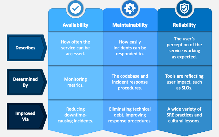
A system should be —
- Reliable
- Scalable
- Maintainable
Reliability means the system should be fault tolerant and working when faults/error happen.
Scalability means should should be able to cater to the growing users, traffic and data
Maintainability means even after adding new functionalities and features as per the new requirements, the system and the existing code should work.
Pic credits : sketchbubble
The Read API in system design is responsible for retrieving data from the system’s database and returning it to the requesting client.
This API is critical for any system that needs to provide access to its data.
Read API can be implemented using the following steps:
- Accepting input: The Read API should accept input from the client about what data is being requested. This input can be in the form of parameters, such as IDs or filters.
- Retrieving data: Once the input is received, the Read API should query the system’s database to retrieve the requested data.
- Formatting data: The Read API should format the data in a way that is easy for the client to understand. This may include converting the data to a specific format, such as JSON or XML.
- Returning data: Finally, the Read API should return the formatted data to the client.
Implementation of a Read API using Python and the Flask web framework:
from flask import Flask, request, jsonify
import sqlite3

app = Flask(__name__)

@app.route('/users')
def get_users():
    # get the query parameters
    name = request.args.get('name')
    age = request.args.get('age')

    # connect to the database
    conn = sqlite3.connect('users.db')
    cursor = conn.cursor()

    # build the SQL query based on the query parameters
    query = "SELECT * FROM users"
    if name:
        query += f" WHERE name = '{name}'"
    if age:
        query += f" AND age = {age}"

    # execute the query and fetch the data
    cursor.execute(query)
    data = cursor.fetchall()

    # format the data as a list of dictionaries
    users = []
    for row in data:
        user = {'id': row[0], 'name': row[1], 'age': row[2]}
        users.append(user)

    # close the database connection
    conn.close()

    # return the formatted data as JSON
    return jsonify(users)
In this implementation, the API accepts query parameters for filtering the users by name and age. It then builds an SQL query based on these parameters and retrieves the data from a SQLite database. The data is then formatted as a list of dictionaries and returned to the client as JSON.
A Write API in system design refers to an API that allows clients to modify or update data in the system. It is often used in systems that require a level of data persistence or require data to be updated in real-time.
In order to implement a Write API, you will need to define the endpoints for the API, the data model for the objects being modified, and the logic for handling incoming requests.
Implementation of a Write API in Python using the Flask framework:
from flask import Flask, request, jsonify
app = Flask(__name__)
# Define the data model for a user
class User:
    def __init__(self, id, name, email):
        self.id = id
        self.name = name
        self.email = email
users = []

# Define the API endpoint for adding a new user
@app.route('/users', methods=['POST'])
def add_user():
    user_data = request.get_json()
    user = User(len(users) + 1, user_data['name'], user_data['email'])
    users.append(user)
    return jsonify({'success': True})# Define the API endpoint for updating an existing user
@app.route('/users/<int:user_id>', methods=['PUT'])
def update_user(user_id):
    user_data = request.get_json()
    user = next((u for u in users if u.id == user_id), None)
    if not user:
        return jsonify({'success': False, 'message': 'User not found'})
    user.name = user_data.get('name', user.name)
    user.email = user_data.get('email', user.email)
    return jsonify({'success': True})if __name__ == '__main__':
    app.run(debug=True)
In this implementation, we define a data model for a user object with an id, name, and email. We also define two API endpoints, one for adding a new user and one for updating an existing user. When a POST request is made to /users, we create a new user object with the data provided in the request, add it to the list of users, and return a JSON response indicating success. When a PUT request is made to_ /users/<user_id>, we look for the user with the specified id in the list of users. If the user is found, we update its name and email properties with the data provided in the request and return a JSON response indicating success. If the user is not found, we return a JSON response indicating failure with a message explaining that the user was not found._
The Search API is a crucial component of many systems, as it allows users to find information quickly and efficiently.
When designing a search API, it’s important to consider the types of queries that users will be performing, as well as the data structures and algorithms that will be used to retrieve results.
Implementation of how a Search API can be implemented using Python:
import json
from typing import List

# assume that the data is already loaded into a list of dictionaries
data = [
    {
        "id": 1,
        "title": "Lorem ipsum",
        "description": "Lorem ipsum dolor sit amet, consectetur adipiscing elit.",
        "tags": ["lorem", "ipsum", "dolor"]
    },
    {
        "id": 2,
        "title": "Dolor sit amet",
        "description": "Dolor sit amet, consectetur adipiscing elit.",
        "tags": ["dolor", "sit", "amet"]
    },
    {
        "id": 3,
        "title": "Consectetur adipiscing elit",
        "description": "Praesent et massa vel ante commodo commodo a eu massa.",
        "tags": ["consectetur", "adipiscing", "elit"]
    }
]def search(query: str) -> List[dict]:
    """
    Search for documents that match the given query
    """
    results = []
    for document in data:
        if query.lower() in document['title'].lower() or query.lower() in document['description'].lower() or query.lower() in [tag.lower() for tag in document['tags']]:
            results.append(document)
    return results# example usage
results = search("Lorem")
print(json.dumps(results, indent=2))
In this implementation, the search API takes a query string as input and returns a list of documents that match the query. The search is performed by iterating through each document in the data list and checking if the query string is present in the document’s title, description, or tags.
A User Info Service is a system component that is responsible for storing and retrieving user information in a system.
It is often a critical component of a larger system because many applications and services rely on user data to function properly.
In a system, the User Info Service would be responsible for managing the following tasks:
- Creating new user accounts
- Authenticating users and validating their credentials
- Retrieving user profile information (e.g. name, email address, profile picture, etc.)
- Updating user profile information
- Deleting user accounts
Implementation of a User Info Service in Python:
class UserInfoService:
    def __init__(self):
        self.users = {}

    def create_user(self, username, password, email):
        if username in self.users:
            raise Exception('User already exists')
        self.users[username] = {
            'password': password,
            'email': email,
            'profile': {}
        }

    def authenticate_user(self, username, password):
        if username not in self.users:
            return False
        return self.users[username]['password'] == password

    def get_user_profile(self, username):
        if username not in self.users:
            return None
        return self.users[username]['profile']

    def update_user_profile(self, username, profile):
        if username not in self.users:
            return False
        self.users[username]['profile'] = profile
        return True

    def delete_user(self, username):
        if username not in self.users:
            return False
        del self.users[username]
        return True
In this implementation, the User Info Service is implemented as a class with methods for each of the tasks described above. The service stores user information in a dictionary, where the keys are usernames and the values are dictionaries containing the user’s password, email, and profile information. The create_user method adds a new user to the dictionary, but first checks to make sure that the username isn't already taken. The authenticate_user method checks whether a given username and password combination is valid. The get_user_profile method retrieves a user's profile information, and the update_user_profile method updates it. Finally, the delete_user method removes a user from the dictionary.
A user graph service is a component in a system design that manages and maintains the relationships between users in a network. It is responsible for storing and updating information about user connections, such as friend lists, followers, or other types of relationships.
This service is commonly used in social networks, online marketplaces, and other systems that require social connections between users.
Implementation of a user graph service using Python and the Flask framework:
from flask import Flask, jsonify, request
from flask_sqlalchemy import SQLAlchemy

app = Flask(__name__)
app.config['SQLALCHEMY_DATABASE_URI'] = 'sqlite:///users.db'
db = SQLAlchemy(app)class User(db.Model):
    id = db.Column(db.Integer, primary_key=True)
    name = db.Column(db.String(50))
    friends = db.relationship('User', secondary='friendships',
        primaryjoin='User.id==friendships.c.user_id',
        secondaryjoin='User.id==friendships.c.friend_id',
        backref=db.backref('friend_of', lazy='dynamic'))friendships = db.Table('friendships',
    db.Column('user_id', db.Integer, db.ForeignKey('user.id')),
    db.Column('friend_id', db.Integer, db.ForeignKey('user.id'))
)@app.route('/users', methods=['GET'])
def get_users():
    users = User.query.all()
    return jsonify([user.name for user in users])@app.route('/users/<int:user_id>', methods=['GET'])
def get_user(user_id):
    user = User.query.get(user_id)
    if user is None:
        return jsonify({'error': 'User not found'})
    return jsonify({'name': user.name, 'friends': [friend.name for friend in user.friends]})@app.route('/users', methods=['POST'])
def create_user():
    name = request.json.get('name')
    user = User(name=name)
    db.session.add(user)
    db.session.commit()
    return jsonify({'id': user.id})@app.route('/users/<int:user_id>/friends', methods=['POST'])
def add_friend(user_id):
    friend_id = request.json.get('friend_id')
    user = User.query.get(user_id)
    friend = User.query.get(friend_id)
    if user is None or friend is None:
        return jsonify({'error': 'User or friend not found'})
    if friend in user.friends:
        return jsonify({'error': 'Already friends'})
    user.friends.append(friend)
    db.session.commit()
    return jsonify({'message': 'Friend added'})if __name__ == '__main__':
    db.create_all()
    app.run()
In this implementation, we use the Flask framework to create a web API for managing users and their connections. We define a User class using SQLAlchemy to represent a user in the system. The User class has a friends relationship that points to other users who are friends of this user. We also define a friendships table that stores the many-to-many relationship between users. This table is used to implement the friends relationship of the User class. The API provides several endpoints for managing users and their connections. The GET /users endpoint returns a list of all users in the system. The GET /users/{id} endpoint returns information about a specific user, including their name and friend list. The POST /users endpoint creates a new user in the system. Finally, the POST /users/{id}/friends endpoint adds a new friend to a user's friend list.
A timeline service in system design is responsible for managing and presenting a chronological list of events or activities.
It can be used in social media platforms, news portals, or other applications where time-based information needs to be presented to users.
Implementation of a timeline service can be done using the following steps:
- Data model: Define the data model for the timeline. This includes the events or activities to be displayed, along with any associated metadata such as timestamps and user IDs.
- Database schema: Create a database schema to store the data model. This can be a relational database such as MySQL or PostgreSQL, or a NoSQL database such as MongoDB or Cassandra.
- API endpoints: Define the API endpoints for the timeline service. This includes endpoints for creating, updating, and deleting events, as well as endpoints for retrieving the events in chronological order.
- Event processing: Define the logic for processing events. This includes verifying user permissions, validating input data, and performing any necessary transformations on the data.
- Presentation: Define the logic for presenting the events to users. This includes sorting the events in chronological order, applying any filters or search queries, and formatting the data for display.
Implementation of a timeline service using Python and the Flask web framework:
from flask import Flask, request, jsonify
import sqlite3

app = Flask(__name__)@app.route('/timeline')
def get_timeline():
    # get the query parameters
    user_id = request.args.get('user_id')
    start_time = request.args.get('start_time')
    end_time = request.args.get('end_time')    # connect to the database
    conn = sqlite3.connect('timeline.db')
    cursor = conn.cursor()    # build the SQL query based on the query parameters
    query = "SELECT * FROM events"
    if user_id:
        query += f" WHERE user_id = {user_id}"
    if start_time and end_time:
        query += f" AND timestamp BETWEEN {start_time} AND {end_time}"
    elif start_time:
        query += f" AND timestamp >= {start_time}"
    elif end_time:
        query += f" AND timestamp <= {end_time}"
    query += " ORDER BY timestamp ASC"    # execute the query and fetch the data
    cursor.execute(query)
    data = cursor.fetchall()    # format the data as a list of dictionaries
    events = []
    for row in data:
        event = {'id': row[0], 'user_id': row[1], 'timestamp': row[2], 'data': row[3]}
        events.append(event)    # close the database connection
    conn.close()    # return the formatted data as JSON
    return jsonify(events)@app.route('/event', methods=['POST'])
def create_event():
    # get the request data
    data = request.get_json()    # validate the data
    if 'user_id' not in data or 'timestamp' not in data or 'data' not in data:
        return jsonify({'error': 'Invalid data'}), 400    # insert the data into the database
    conn = sqlite3.connect('timeline.db')
    cursor = conn.cursor()
    query = "INSERT INTO events (user_id, timestamp, data) VALUES (?, ?, ?)"
    cursor.execute(query, (data['user_id'], data['timestamp'], data['data']))
    conn.commit()
    event_id = cursor.lastrowid
    conn.close()    # return the ID of the created event
    return jsonify({'id': event_id}), 201
In this implementation, the timeline service provides two endpoints. The get_timeline() endpoint retrieves events from the database based on query parameters for user ID.
A notification service in system design is a mechanism that allows a system to send notifications to users or other systems about events or changes in the system.
It is often used in systems that require real-time updates or event-driven architectures. In order to implement a notification service, you will need to define the message format, the delivery mechanism, and the logic for handling incoming notifications.
Implementation of a notification service in Python using the Flask framework and the Redis Pub/Sub messaging system:
from flask import Flask, request
import redis

app = Flask(__name__)
redis_client = redis.Redis(host='localhost', port=6379)# Define the API endpoint for sending notifications
@app.route('/notifications', methods=['POST'])
def send_notification():
    notification_data = request.get_json()
    channel = notification_data['channel']
    message = notification_data['message']
    redis_client.publish(channel, message)
    return 'Notification sent'# Define the function for handling incoming notifications
def handle_notification(channel, message):
    print(f'Received message on channel {channel}: {message}')if __name__ == '__main__':
    # Subscribe to the 'notifications' channel and start listening for messages
    pubsub = redis_client.pubsub()
    pubsub.subscribe('notifications')
    for message in pubsub.listen():
        handle_notification(message['channel'], message['data'])
In this implementation, we define an API endpoint for sending notifications with a channel and message payload. When a POST request is made to /notifications, we publish the message to the Redis Pub/Sub system using the specified channel. We also define a function for handling incoming notifications. This function simply prints the channel and message payload to the console, but in a real system, you would likely use this function to trigger some kind of action or update in the system. Finally, we subscribe to the ‘notifications’ channel using the Redis pubsub() method and start listening for messages. When a message is received, the handle_notification() function is called with the channel and message payload as arguments._
A full text search service in system design is a mechanism that allows a system to search for and retrieve documents or other data based on keyword or phrase searches.
It is often used in systems that have large amounts of unstructured or semi-structured data, such as text documents or web pages. In order to implement a full text search service, you will need to define the data model and indexing strategy, the search API, and the logic for querying and retrieving results.
Implementation of a full text search service in Python using the Flask framework and the Elasticsearch search engine:
from flask import Flask, request, jsonify
from elasticsearch import Elasticsearch

app = Flask(__name__)
es = Elasticsearch()# Define the data model for a document
class Document:
    def __init__(self, id, title, content):
        self.id = id
        self.title = title
        self.content = content# Define the function for indexing documents
def index_document(document):
    es.index(index='documents', body={
        'id': document.id,
        'title': document.title,
        'content': document.content
    })# Define the API endpoint for searching documents
@app.route('/search', methods=['GET'])
def search_documents():
    query = request.args.get('q', '')
    results = es.search(index='documents', body={
        'query': {
            'multi_match': {
                'query': query,
                'fields': ['title', 'content']
            }
        }
    })['hits']['hits']
    documents = [Document(r['_source']['id'], r['_source']['title'], r['_source']['content']) for r in results]
    return jsonify({'documents': [doc.__dict__ for doc in documents]})if __name__ == '__main__':
    # Index some example documents
    documents = [
        Document(1, 'Lorem Ipsum', 'Lorem ipsum dolor sit amet, consectetur adipiscing elit.'),
        Document(2, 'Python Tutorial', 'Learn Python programming with this tutorial.'),
        Document(3, 'Flask Web Framework', 'Build web applications with Flask.')
    ]
    for doc in documents:
        index_document(doc)
    app.run(debug=True)
In this implementation, we define a data model for a document object with an id, title, and content. We also define a function for indexing documents in the Elasticsearch search engine. When a GET request is made to /search?q=, we use the Elasticsearch search API to search for documents containing the specified query in either the title or content fields. We then construct a list of Document objects from the search results and return them as a JSON response. Finally, we index some example documents in the Elasticsearch index when the application starts up._
Caching is a technique used to store frequently accessed data in a temporary storage area so that it can be retrieved faster when required. It is commonly used in system design to improve performance and reduce latency.
How Caching Works:
Caching works by storing data in a fast-access storage area that is close to the data consumer. When data is requested, the system checks the cache first to see if the data is already available. If the data is available in the cache, it is retrieved and returned to the consumer. If the data is not available in the cache, the system retrieves the data from the original source and stores it in the cache for future use.
Implementing a Caching Service with Python:
In Python, we can implement a caching service using the built-in dict data type.
Implementation of a caching service that stores the result of a function call using a dictionary:
cache = {}

def cached_func(func):
    def wrapper(*args):
        if args in cache:
            return cache[args]
        else:
            result = func(*args)
            cache[args] = result
            return result
    return wrapper
In this implementation, cache is a dictionary that will be used to store the results of function calls. The cached_func decorator takes a function as an argument and returns a new function that caches the results of the original function. The new function, wrapper, first checks the cache to see if the result of the function call has already been computed. If the result is available in the cache, it is returned immediately. If the result is not in the cache, the original function is called with the arguments provided, and the result is stored in the cache before being returned._
To use the caching service, we simply decorate the function we want to cache with the cached_func decorator:
@cached_func
def fibonacci(n):
    if n <= 1:
        return n
    else:
        return fibonacci(n-1) + fibonacci(n-2)
In this implementation, the fibonacci function will be cached, so that subsequent calls to fibonacci(n) with the same value of n will return the cached result instead of computing the result again. Caching can greatly improve the performance of a system by reducing the time needed to compute frequently accessed data. However, it’s important to be aware of the limitations of caching, such as the increased memory usage and the need to keep the cache consistent with the original data source.
It’s the process of distributing requests or messages from a single source to multiple destinations.
This is a common pattern in distributed systems, where a service or application needs to send information to multiple downstream systems.
One way to implement a fan out service is to use a message queue. The service would receive requests or messages from the source system, and then publish those messages to a message queue. Each downstream system would then subscribe to the message queue and receive a copy of the message.
Implementation of a fan out service using Python and RabbitMQ as the message queue:
import pika

# Connect to RabbitMQ
connection = pika.BlockingConnection(pika.ConnectionParameters('localhost'))
channel = connection.channel()# Create the message queue
channel.exchange_declare(exchange='fanout_exchange', exchange_type='fanout')# Define the message to be sent
message = 'Hello, world!'# Publish the message to the message queue
channel.basic_publish(exchange='fanout_exchange', routing_key='', body=message)# Close the connection
connection.close()
In this implementation, the service connects to a RabbitMQ instance running on localhost. It then declares a fanout exchange, which is a type of exchange that broadcasts messages to all bound queues. The service then creates a message to be sent and publishes it to the exchange with an empty routing key, indicating that the message should be sent to all queues bound to the exchange.
To receive the messages, downstream systems would need to create a queue and bind it to the fanout exchange.
Here’s an implementation of a downstream system using Python and RabbitMQ:
import pika

# Connect to RabbitMQ
connection = pika.BlockingConnection(pika.ConnectionParameters('localhost'))
channel = connection.channel()# Create a queue and bind it to the fanout exchange
result = channel.queue_declare(queue='', exclusive=True)
queue_name = result.method.queue
channel.queue_bind(exchange='fanout_exchange', queue=queue_name)# Define a callback function to handle received messages
def callback(ch, method, properties, body):
    print(f'Received message: {body}')# Start consuming messages from the queue
channel.basic_consume(queue=queue_name, on_message_callback=callback, auto_ack=True)
channel.start_consuming()
In this implementation, the downstream system connects to the same RabbitMQ instance as the fan out service. It then declares a queue with an empty name, which creates a unique queue name that is only accessible to the current connection. The downstream system then binds the queue to the fanout exchange created by the fan out service. The system defines a callback function to handle received messages, which simply prints the message body to the console. Finally, the system starts consuming messages from the queue using the basic_consume method, passing the callback function as an argument.
A memory cache is a system component that stores frequently accessed data in memory for fast access. It can be used to improve the performance of a system by reducing the number of expensive database queries or other resource-intensive operations.
In a system, the memory cache would be responsible for managing the following tasks:
- Storing and retrieving data from memory
- Expiring or invalidating cached data after a certain amount of time or under certain conditions
- Maintaining cache consistency and preventing data corruption
- Managing cache capacity to avoid running out of memory
Implementation of a simple memory cache in Python:
class MemoryCache:
    def __init__(self, capacity=1000, default_ttl=60):
        self.cache = {}
        self.capacity = capacity
        self.default_ttl = default_ttl

    def get(self, key):
        if key not in self.cache:
            return None

        value, expiration = self.cache[key]
        if expiration is not None and expiration < time.time():
            del self.cache[key]
            return None

        return value

    def set(self, key, value, ttl=None):
        if len(self.cache) >= self.capacity:
            self.evict()

        if ttl is None:
            ttl = self.default_ttl

        expiration = time.time() + ttl
        self.cache[key] = (value, expiration)

    def delete(self, key):
        if key in self.cache:
            del self.cache[key]

    def evict(self):
        now = time.time()
        expired_keys = [k for k, (v, e) in self.cache.items() if e is not None and e < now]
        for key in expired_keys:
            del self.cache[key]

    def clear(self):
        self.cache.clear()
In this implementation, the MemoryCache class uses a dictionary to store key-value pairs, where the keys are the data being cached and the values are tuples containing the cached value and its expiration time. The get method retrieves a value from the cache, checking its expiration time to ensure it hasn't expired. The set method adds a new key-value pair to the cache, setting an optional time-to-live (TTL) value to determine how long the value should be cached for. If the cache is at capacity, the evict method is called to remove expired keys and make room for new ones. The delete method removes a key-value pair from the cache, and the clear method removes all key-value pairs from the cache.
DNS (Domain Name System) is a system used to translate human-readable domain names into IP addresses. It acts as a directory for the internet, allowing users to easily access websites and other internet services without needing to remember IP addresses.
In a system, a DNS server would be responsible for managing the following tasks:
- Resolving domain names into IP addresses
- Caching resolved IP addresses to improve performance
- Load balancing between multiple IP addresses for a given domain name
- Handling domain name registration and management
Implementation of a simple DNS resolver in Python:
import socket

class DNSResolver:
    def __init__(self, ttl=60):
        self.cache = {}
        self.ttl = ttl

    def resolve(self, domain):
        if domain in self.cache:
            ip, expiration = self.cache[domain]
            if expiration > time.time():
                return ip

        ips = socket.getaddrinfo(domain, None)
        if not ips:
            return None

        ip = ips[0][4][0]
        self.cache[domain] = (ip, time.time() + self.ttl)
        return ip

    def clear_cache(self):
        self.cache.clear()
In this implementation, the DNSResolver class uses the socket module to resolve domain names into IP addresses. The resolve method first checks the cache to see if the requested domain name has already been resolved and cached. If the cached IP address has not expired, it is returned immediately. Otherwise, the getaddrinfo function is called to resolve the domain name into one or more IP addresses. If no IP addresses are returned, None is returned. Otherwise, the first IP address in the list is returned and cached with an expiration time based on the TTL value specified in the constructor. The clear_cache method removes all cached IP addresses from the cache.
Real-time message ingestion is the process of capturing and processing messages as they are generated in real-time.
This is a common requirement for many systems that handle real-time data, such as chat applications, social media platforms, and IoT systems.
In a system, real-time message ingestion would be responsible for managing the following tasks:
- Capturing messages as they are generated
- Storing messages in a way that allows for efficient retrieval and querying
- Processing messages in real-time to perform actions such as notifications or real-time analytics
- Scaling to handle high message volume and ensure high availability
Implementation of a simple real-time message ingestion system in Python using the Flask web framework and Redis as a message broker:
from flask import Flask, request
from redis import Redis
import json

app = Flask(__name__)
redis = Redis(host='localhost', port=6379)@app.route('/message', methods=['POST'])
def add_message():
    message = json.loads(request.data)
    redis.publish('messages', json.dumps(message))
    return 'Message received'if __name__ == '__main__':
    app.run(debug=True)
In this implementation, the Flask web framework is used to create an HTTP endpoint at /message that accepts JSON-formatted messages via a POST request. The add_message function deserializes the JSON payload, and then publishes the message to a Redis message broker using the publish method. This allows the message to be distributed to any number of subscribers in real-time.
Subscribers can then use Redis’ subscribe method to listen for messages on the 'messages' channel:
from redis import Redis
import json

redis = Redis(host='localhost', port=6379)
pubsub = redis.pubsub()
pubsub.subscribe('messages')for message in pubsub.listen():
    if message['type'] == 'message':
        data = json.loads(message['data'])
        # Do something with the message data
In this implementation, the pubsub object is created to listen for messages on the 'messages' channel. The listen method blocks until a message is received, and then returns a dictionary with the message type and data. If the message type is 'message', the message data is deserialized from JSON and can then be used for further processing.
A load balancer is a system component that distributes incoming network traffic across multiple servers to improve performance, reliability, and availability.
Load balancers can be used to handle a large number of requests, prevent overload on individual servers, and ensure that traffic is distributed evenly among servers.
In a system, a load balancer would be responsible for managing the following tasks:
- Monitoring server health and availability
- Distributing traffic across available servers
- Managing session persistence (i.e. ensuring that subsequent requests from a client are routed to the same server)
- Handling SSL termination (i.e. decrypting encrypted traffic and forwarding it to the appropriate server)
Implementation of a simple load balancer in Python:
import random
class LoadBalancer:
    def __init__(self, servers):
        self.servers = servers
        self.num_servers = len(servers)
        self.server_statuses = [True] * self.num_servers

    def choose_server(self):
        available_servers = [i for i in range(self.num_servers) if self.server_statuses[i]]
        if not available_servers:
            return None
        return random.choice(available_servers)

    def handle_request(self, request):
        server_index = self.choose_server()
        if server_index is None:
            raise Exception("No available servers")
        server = self.servers[server_index]
        return server.handle_request(request)

    def set_server_status(self, server_index, status):
        self.server_statuses[server_index] = status
In this implementation, the LoadBalancer class takes a list of Server objects in its constructor. The choose_server method randomly selects an available server from the list, based on the current server statuses. The handle_request method uses the choose_server method to select a server, and then forwards the request to that server's handle_request method. If no available server is found, an exception is raised. The set_server_status method is used to set the status of a server to either available or unavailable.
A Content Delivery Network (CDN) is a distributed network of servers that helps to deliver content faster and more efficiently to end-users by caching content closer to the user’s location.
A CDN can be used in a system design to improve website performance and reliability by reducing latency, improving website availability and scalability, and reducing bandwidth costs.
Implementation of CDN using Amazon CloudFront, one of the popular CDN services available:
- Sign up for an AWS account and create a new CloudFront distribution.
aws cloudfront create-distribution \
    --origin-domain-name example.com \
    --default-root-object index.html \
    --enabled
- Set up your origin server(s) by creating an Amazon S3 bucket or an EC2 instance as your origin server.
- Create a new DNS record for your distribution using your preferred DNS provider (e.g., Amazon Route 53) and point it to your CloudFront distribution.
- Test your CDN by accessing your website using the new DNS record. You should see improved performance and faster load times.
In summary, implementing a CDN in a system design can greatly improve website performance and reliability by caching content closer to end-users. It can also reduce latency, improve website availability and scalability, and reduce bandwidth costs.
A job server in system design is responsible for managing and executing background jobs or tasks asynchronously. It can be used in various applications such as web scraping, data processing, or batch processing.
The implementation of a job server can be done using the following steps:
- Job queue: Define a job queue to store the jobs to be executed. This can be a message queue such as RabbitMQ, a database table, or a simple in-memory data structure such as a list.
- Job producer: Define a job producer to add jobs to the job queue. This can be a user interface, a REST API endpoint, or any other application logic that generates jobs.
- Job consumer: Define a job consumer to fetch jobs from the job queue and execute them. This can be a worker process that runs continuously in the background, or a scheduler that runs periodically to check for new jobs.
- Job executor: Define the logic for executing the jobs. This includes processing input data, performing the necessary calculations or operations, and generating output data.
Implementation of a job server using Python and the Flask web framework:
from flask import Flask, request, jsonify
from queue import Queue
import threading

app = Flask(__name__)
job_queue = Queue()def worker():
    while True:
        job = job_queue.get()
        # execute the job logic here
        print(f"Executing job {job['id']} with data {job['data']}")
        job_queue.task_done()@app.route('/job', methods=['POST'])
def create_job():
    # get the request data
    data = request.get_json()    # validate the data
    if 'data' not in data:
        return jsonify({'error': 'Invalid data'}), 400    # add the job to the job queue
    job_id = len(job_queue) + 1
    job = {'id': job_id, 'data': data['data']}
    job_queue.put(job)    # return the ID of the created job
    return jsonify({'id': job_id}), 201if __name__ == '__main__':
    # start the worker threads
    for i in range(4):
        t = threading.Thread(target=worker)
        t.daemon = True
        t.start()    # start the Flask app
    app.run(debug=True)
In this implementation, the job server provides a single endpoint create_job() that accepts job data as input and adds it to the job queue. The worker() function runs continuously in the background, fetching jobs from the queue and executing them. To start the worker threads, the name == 'main'_ block creates four worker threads and starts them in daemon mode. This ensures that the threads will exit gracefully when the main thread terminates. When a job is added to the job queue, it is assigned an ID and a dictionary object with the job data. The worker thread fetches the job from the queue, extracts the job data, and executes the job logic. In this example, the job logic is simply printing the job ID and data to the console, but it could be any arbitrary code for processing the job data. Finally, the worker thread calls task_done() to signal that the job has been completed.
Workers in system design refer to background processes that perform tasks asynchronously and independently of the main system flow.
They are often used to perform tasks that are time-consuming or resource-intensive, such as processing large files, sending emails, or performing data analysis.
Implementation of a worker system in Python using the Celery distributed task queue:
from celery import Celery
import time

app = Celery('tasks', broker='pyamqp://guest@localhost//')# Define a task that takes some time to complete
@app.task
def long_task(duration):
    time.sleep(duration)
    return f'Task completed after {duration} seconds'if __name__ == '__main__':
    # Queue up some tasks
    result1 = long_task.delay(5)
    result2 = long_task.delay(10)
    result3 = long_task.delay(15)    # Check the status of the tasks
    print(f'Task 1 status: {result1.status()}')
    print(f'Task 2 status: {result2.status()}')
    print(f'Task 3 status: {result3.status()}')    # Wait for the tasks to complete and retrieve the results
    print(result1.get())
    print(result2.get())
    print(result3.get())
In this implementation, we define a Celery app and a task that takes a specified number of seconds to complete using the time.sleep() function. We also define a main function that queues up some example tasks and checks their status before waiting for them to complete and retrieving the results. When the application runs, the long_task() function is executed asynchronously and independently of the main system flow. We can queue up multiple tasks and check their status using the result.status() method. We can also retrieve the results of the completed tasks using the result.get() method.
An application server in system design is a server that provides a platform for running and managing applications, often in a distributed or scalable environment.
It typically includes features such as load balancing, caching, and session management, and is often used to deploy web applications or APIs.
Implementation of an application server in Python using the Flask web framework and the Gunicorn WSGI HTTP server:
from flask import Flask, jsonify
import os

app = Flask(__name__)# Define an API endpoint
@app.route('/api', methods=['GET'])
def hello():
    return jsonify({'message': 'Hello, world!'})if __name__ == '__main__':
    # Get the port number from the environment variable, or use a default value
    port = int(os.environ.get('PORT', 5000))
    # Run the application using the Gunicorn WSGI HTTP server
    app.run(host='0.0.0.0', port=port)
In this implementation, we define a Flask app with a single API endpoint that returns a JSON response. We then use the Gunicorn HTTP server to run the app on a specified port. We also get the port number from an environment variable, which allows us to easily configure the port when deploying the app.
To run this application, you would first need to install Flask and Gunicorn. You can do this using pip:
pip install flask gunicorn
Once you have installed the necessary packages, you can run the application using the following command:
Copy code
gunicorn app:app
This command tells Gunicorn to run the app module (which contains our Flask app) and the app variable (which is the name of our Flask app). Gunicorn will start up multiple worker processes to handle incoming requests, and will handle load balancing and other features automatically.
Queues are an important part of many system designs, allowing you to process tasks and messages in a distributed or asynchronous manner.
In this , we’ll implement a simple queue using the Python queue module.
import queue
import time
import threading

# Define a function that will process items from the queue
def process_queue(q):
    while True:
        item = q.get()
        print(f'Processing item {item}...')
        time.sleep(1)
        q.task_done()# Create a queue and start the worker threads
q = queue.Queue()
for i in range(5):
    t = threading.Thread(target=process_queue, args=(q,))
    t.daemon = True
    t.start()# Add some items to the queue
for i in range(10):
    q.put(i)# Wait for the queue to be processed
q.join()
print('All items processed')
In this implementation, we define a process_queue() function that will process items from the queue. We then create a queue.Queue() object and start five worker threads that will call process_queue() to process items from the queue. We then add ten items to the queue using q.put(). The worker threads will automatically process these items in a first-in, first-out (FIFO) order. Finally, we call_ q.join() to wait for all of the items to be processed. This function blocks until all items in the queue have been processed and marked as done using q.task_done()._
Object storage is a method of storing and retrieving unstructured data in the form of objects. It is often used to store large amounts of data, such as media files, and can be accessed over a network using APIs.
How an object store can be implemented using Python:
import os
import hashlib

class ObjectStore:
    def __init__(self, storage_directory):
        self.storage_directory = storage_directory    def put(self, data):
        """
        Store an object in the object store
        """
        # generate a unique filename for the object
        filename = hashlib.md5(data).hexdigest()        # write the object data to a file
        with open(os.path.join(self.storage_directory, filename), 'wb') as f:
            f.write(data)        return filename    def get(self, filename):
        """
        Retrieve an object from the object store
        """
        # read the object data from a file
        with open(os.path.join(self.storage_directory, filename), 'rb') as f:
            data = f.read()        return data# example usage
object_store = ObjectStore('/path/to/storage/directory')
data = b'This is some test data'
filename = object_store.put(data)
retrieved_data = object_store.get(filename)
print(retrieved_data)
In this implementation, the object store is implemented as a Python class with two methods: put and get. The_ put method takes an object as input, generates a unique filename for the object using a hash function, and writes the object data to a file in the specified storage directory. The method returns the generated filename, which can be used to retrieve the object later. The get method takes a filename as input and reads the corresponding object data from a file in the storage directory. The method returns the object data as bytes.
Authentication is the process of verifying the identity of a user, typically by requiring them to provide credentials such as a username and password.
It is a crucial component of many systems to ensure that only authorized users can access protected resources.
How authentication can be implemented in Python using the Flask web framework:
from flask import Flask, request, jsonify

app = Flask(__name__)# mock user data for demonstration purposes
users = {
    "alice": {
        "password": "password123",
        "email": "alice@example.com"
    },
    "bob": {
        "password": "password456",
        "email": "bob@example.com"
    }
}# authentication endpoint
@app.route('/authenticate', methods=['POST'])
def authenticate():
    username = request.json.get('username')
    password = request.json.get('password')    if username in users and password == users[username]['password']:
        # authentication successful
        return jsonify({'success': True, 'email': users[username]['email']})
    else:
        # authentication failed
        return jsonify({'success': False, 'message': 'Invalid username or password'}), 401# example usage
response = app.test_client().post('/authenticate', json={'username': 'alice', 'password': 'password123'})
print(response.get_json())
In this implementation, the authentication process is implemented as a Flask endpoint that accepts a username and password as input in a JSON payload. The endpoint checks the provided credentials against a mock user database, and if they are valid, returns a JSON response indicating success along with the user’s email address. If the credentials are invalid, the endpoint returns a JSON response indicating failure along with an error message and a 401 HTTP status code to indicate unauthorized access. In a real-world system, authentication would likely involve more sophisticated mechanisms such as encryption, multi-factor authentication, and user management.
Batch processing is a method of processing a large number of input items as a single batch, typically for efficiency reasons.
It is often used in systems that need to process large amounts of data, such as data pipelines or ETL (Extract, Transform, Load) processes.
How batch processing can be implemented in Python using the multiprocessing module:
import multiprocessing

def process_batch(batch):
    """
    Process a single batch of input items
    """
    # process the input items in the batch
    result = []
    for item in batch:
        result.append(item.upper())    return resultdef batch_process(input_data, batch_size=10):
    """
    Process the input data in batches
    """
    # split the input data into batches
    batches = [input_data[i:i+batch_size] for i in range(0, len(input_data), batch_size)]    # process each batch using multiprocessing
    with multiprocessing.Pool() as pool:
        results = pool.map(process_batch, batches)    # flatten the results and return them
    return [item for batch_result in results for item in batch_result]# example usage
input_data = ['apple', 'banana', 'cherry', 'date', 'elderberry', 'fig', 'grape', 'honeydew', 'kiwi', 'lemon']
output_data = batch_process(input_data, batch_size=3)
print(output_data)
In this implementation, the batch_process function takes a list of input items and a batch size as input, and splits the input items into batches of the specified size. It then uses the multiprocessing module to process each batch in parallel using the process_batch function, which simply applies a transformation to each item in the batch. Finally, the results from each batch are combined into a single output list and returned.
Cloud storage is a method of storing data in a remote server or a network of servers that are accessible over the internet.
It is commonly used in systems that require scalable, flexible, and reliable storage solutions.
How cloud storage can be implemented in Python using the boto3 library to interact with Amazon S3:
import boto3

# create an S3 client
s3 = boto3.client('s3')# create a new bucket
bucket_name = 'my-bucket'
s3.create_bucket(Bucket=bucket_name)# upload a file to the bucket
file_name = 'example.txt'
with open(file_name, 'rb') as f:
    s3.upload_fileobj(f, bucket_name, file_name)# download a file from the bucket
with open('downloaded.txt', 'wb') as f:
    s3.download_fileobj(bucket_name, file_name, f)# list the contents of the bucket
response = s3.list_objects_v2(Bucket=bucket_name)
for item in response['Contents']:
    print(item['Key'])
In this implementation, the boto3 library is used to create an S3 client that can interact with Amazon S3. A new bucket is created using the create_bucket method, and a file is uploaded to the bucket using the upload_fileobj method. The file is then downloaded from the bucket using the download_fileobj method, and the contents of the bucket are listed using the list_objects_v2 method.
Stream processing is a critical component of many modern system designs, allowing applications to process large volumes of data in real-time. In stream processing, data is processed as it is generated, allowing for faster analysis and insights.
Implementation of stream processing using Python and Apache Kafka:
- Set up Apache Kafka using the Confluent platform, which provides a Python client for interacting with Kafka:
from confluent_kafka import Producer, Consumer

conf = {
    'bootstrap.servers': 'my-kafka-broker:9092',
    'client.id': 'my-client-id'
}producer = Producer(conf)
consumer = Consumer({
    'bootstrap.servers': 'my-kafka-broker:9092',
    'group.id': 'my-consumer-group',
    'auto.offset.reset': 'earliest'
})- Create a Kafka topic to store the incoming stream of data:
producer.produce('my-topic', key='key', value='value')
- Set up a Kafka consumer to process the incoming stream of data:
consumer.subscribe(['my-topic'])

while True:
    msg = consumer.poll(1.0)    if msg is None:
        continue    if msg.error():
        print(f"Consumer error: {msg.error()}")
continue print(f"Received message: {msg.value().decode('utf-8')}")- Process the incoming stream of data using Python’s data processing libraries like pandas, numpy, or scikit-learn:
import pandas as pd

df = pd.read_json(msg.value())
# perform data processing on the DataFrame

*   Write the processed data to an output stream or database:

import sqlite3

conn = sqlite3.connect('my-db')
c = conn.cursor()# create table if it doesn't exist
c.execute('''CREATE TABLE IF NOT EXISTS my_table
             (column1 text, column2 text, column3 text)''')# insert data into table
c.execute(f"INSERT INTO my_table VALUES (?, ?, ?)", (val1, val2, val3))
conn.commit()# close database connection
conn.close()
In summary, stream processing using Python and Apache Kafka is a powerful tool for system design, allowing for the real-time processing of large volumes of data. The above code shows how to set up a Kafka producer to send data to a topic, a consumer to read data from the topic, process the data using data processing libraries, and write the results to an output stream or database.
Master-Slave is a common pattern used in system design to improve the scalability, performance, and availability of applications.
In this pattern, there is one master node that handles write requests and one or more slave nodes that handle read requests.
Here’s an implementation of the Master-Slave pattern using Python and Redis:
- Set up Redis using the redis-py library:
import redis

# Connect to Redis as the master node
master = redis.Redis(host='my-master-redis-host', port=6379)# Connect to Redis as the slave node(s)
slave1 = redis.Redis(host='my-slave-redis-host-1', port=6379)
slave2 = redis.Redis(host='my-slave-redis-host-2', port=6379)

*   Write data to the master node using the `set()` method:

master.set('my-key', 'my-value')

*   Read data from the slave node(s) using the `get()` method:

# read from slave1
value = slave1.get('my-key')

# if value is None, try reading from slave2
if value is None:
    value = slave2.get('my-key')

*   Configure Redis to replicate data from the master to the slave nodes:

# Set up Redis as a master-slave replication system
master_config = {
    'slaveof': None  # master has no slave
}

slave1_config = {
    'slaveof': ('my-master-redis-host', 6379)
}slave2_config = {
    'slaveof': ('my-master-redis-host', 6379)
}# Configure the Redis instances
master.config_set(**master_config)
slave1.config_set(**slave1_config)
slave2.config_set(**slave2_config)
In summary, implementing the Master-Slave pattern using Python and Redis is a powerful tool for system design, allowing for the improved scalability, performance, and availability of applications. The above code shows how to set up Redis as a master-slave replication system, write data to the master node, and read data from the slave node(s).
Authentication servers are a critical component of many modern system designs, allowing applications to authenticate users and manage access control. In this pattern, there is a separate server dedicated to handling authentication requests and managing user credentials.
Here’s an implementation of an authentication server using Python and Flask:
- Set up a Flask server to handle authentication requests:
from flask import Flask, request, jsonify

app = Flask(__name__)@app.route('/login', methods=['POST'])
def login():
    # Authenticate the user
    username = request.json.get('username')
    password = request.json.get('password')

    # Check the username and password against the database
    if authenticate_user(username, password):
        # If the user is authenticated, generate a token
        token = generate_token(username)
        return jsonify({'token': token})
    else:
return jsonify({'error': 'Invalid username or password'})- Set up a user database to store user credentials:
import sqlite3

def create_user_table():
    conn = sqlite3.connect('users.db')
    c = conn.cursor()
    c.execute('''CREATE TABLE IF NOT EXISTS users
                 (username text, password text)''')
    conn.commit()
    conn.close()def add_user(username, password):
    conn = sqlite3.connect('users.db')
    c = conn.cursor()
    c.execute(f"INSERT INTO users VALUES (?, ?)", (username, password))
    conn.commit()
    conn.close()def authenticate_user(username, password):
    conn = sqlite3.connect('users.db')
    c = conn.cursor()
    c.execute(f"SELECT * FROM users WHERE username = '{username}' AND password = '{password}'")
    result = c.fetchone()
    conn.close()
return result is not None- Set up a token generation method to generate and validate authentication tokens:
import jwt

JWT_SECRET_KEY = 'my-secret-key'def generate_token(username):
    payload = {'username': username}
    return jwt.encode(payload, JWT_SECRET_KEY, algorithm='HS256')def validate_token(token):
    try:
        decoded_payload = jwt.decode(token, JWT_SECRET_KEY, algorithms=['HS256'])
        return decoded_payload.get('username')
    except jwt.exceptions.DecodeError:
return None- Set up an access control mechanism to check user authentication:
from functools import wraps

def auth_required(f):
    @wraps(f)
    def decorated_function(*args, **kwargs):
        token = request.headers.get('Authorization')
        if token is None:
            return jsonify({'error': 'Authentication required'}), 401        username = validate_token(token)
        if username is None:
            return jsonify({'error': 'Invalid token'}), 401        return f(*args, **kwargs)    return decorated_function
In summary, implementing an authentication server using Python and Flask is a powerful tool for system design, allowing for the authentication and access control of users in a scalable and secure manner. The above code shows how to set up a Flask server to handle authentication requests, set up a user database to store user credentials, generate and validate authentication tokens, and set up an access control mechanism to check user authentication.
SQL Read replicas are an important tool for system design that can help improve the performance, scalability, and availability of databases. A read replica is a copy of a database that can be used to offload read requests from the primary database, reducing its load and improving its performance.
Here is an implementation of SQL Read replicas using Python and Amazon Web Services (AWS):
- Create an AWS account and configure the AWS credentials using the Boto3 library:
import boto3

session = boto3.Session(
    aws_access_key_id='YOUR_ACCESS_KEY',
    aws_secret_access_key='YOUR_SECRET_KEY',
    region_name='YOUR_REGION'
)- Connect to the primary database using the SQL Alchemy library:
from sqlalchemy import create_engine

primary_db_uri = 'postgresql://user:password@primary-db-host:port/primary_db_name'
primary_engine = create_engine(primary_db_uri)- Create a read replica using the AWS RDS service and the Boto3 library:
client = session.client('rds')

response = client.create_db_instance_read_replica(
    DBInstanceIdentifier='my-read-replica',
    SourceDBInstanceIdentifier='my-primary-db',
    DBInstanceClass='db.t2.micro',
    AvailabilityZone='us-west-2a',
    PubliclyAccessible=False,
    Tags=[
        {
            'Key': 'Name',
            'Value': 'my-read-replica'
        }
    ]
)read_replica_endpoint = response['DBInstance']['Endpoint']['Address']- Connect to the read replica database using the SQL Alchemy library:
read_replica_uri = f"postgresql://user:password@{read_replica_endpoint}:port/read_replica_db_name"
read_replica_engine = create_engine(read_replica_uri)- Offload read requests to the read replica using SQL Alchemy’s
create_session()method:
from sqlalchemy.orm import sessionmaker

Session = sessionmaker(bind=read_replica_engine)# create a session using the read replica engine
session = Session()# perform read requests using the session
result = session.execute('SELECT * FROM my_table')
In summary, implementing SQL Read replicas using Python and AWS is a straightforward process. The above code shows how to create a read replica database using the Boto3 library, connect to it using the SQL Alchemy library, and offload read requests to it using a session. This can help improve the performance, scalability, and availability of databases in system design.
Load and load estimation are important concepts in system design, as they help engineers determine the resources and capacity required to handle the anticipated workload for a system.
- Load: Load refers to the amount of work or resource utilization that a system is handling at a given time. It can be measured in terms of the number of requests per second, CPU utilization, memory usage, disk I/O, network traffic, or any other relevant metric.
- Load Estimation: Load estimation is the process of predicting the future load on a system. This involves analyzing the patterns of resource utilization, user behavior, and business requirements to determine the expected workload. Load estimation helps engineers to design a system that can handle the anticipated load and avoid overloading or underutilization.
Implementation of load and load estimation in system design using Python:
import psutil
import time

# Define the function to calculate system load
def get_system_load():
    # Get the current system load
    load = psutil.cpu_percent()    # Wait for 1 second to get a more accurate reading
    time.sleep(1)    # Calculate the average system load over the past 1 second
    load = psutil.cpu_percent()    return load# Define the function to estimate future system load
def estimate_load():
    # Get the current system load
    current_load = get_system_load()    # Predict the future system load based on historical data
    predicted_load = current_load * 2    return predicted_load
In this implementation, we use the psutil library to get the current CPU load of the system. We define a function called get_system_load() which calculates the average system load over the past 1 second. We use a time.sleep(1) call to wait for 1 second before calculating the load, in order to get a more accurate reading.
We then define a function called estimate_load() which calls get_system_load() to get the current system load, and then predicts the future system load based on historical data. In this example, we simply double the current system load to estimate the future load, but in a real system design, more complex algorithms and historical data could be used to make more accurate predictions.
To estimate the performance of the system you have designed, there are many metrics. In this we will cover most important three —
- Throughput — Its measured by no of jobs processed/ second
- Response time — Its measured by the time between sending request and getting a response
- Latency — Its measured by the time it takes for a request waiting in the queue to be completed.
Throughput: Throughput is a measure of the rate at which a system can process requests.
Implementation of throughput in system design using Python:
import time

# Define the function to measure throughput
def measure_throughput(num_requests):
    start_time = time.time()    # Perform the requests
    for i in range(num_requests):
        perform_request()    end_time = time.time()
    elapsed_time = end_time - start_time    # Calculate the throughput
    throughput = num_requests / elapsed_time    return throughput
In this implementation, we define a function called measure_throughput() which takes the number of requests as an argument, and measures the time it takes to perform the requests using the time library. We then calculate the throughput by dividing the number of requests by the elapsed time.
Response time: Response time is a measure of the time it takes for a system to respond to a request.
Implementation of response time in system design using Python:
import time

# Define the function to measure response time
def measure_response_time():
    start_time = time.time()    # Perform the request
    response = perform_request()    end_time = time.time()
    elapsed_time = end_time - start_time    # Log the response time
    log_response_time(elapsed_time)    return response
In this example, we define a function called measure_response_time() which measures the time it takes to perform a single request using the time library. We then log the response time for debugging and performance analysis purposes.
Latency: Latency is a measure of the time it takes for a request to be processed by a system.
Implementation of latency in system design using Python:
import time

# Define the function to measure latency
def measure_latency(num_requests):
    start_time = time.time()    # Perform the requests
    for i in range(num_requests):
        start_request_time = time.time()
        perform_request()
        end_request_time = time.time()
        elapsed_request_time = end_request_time - start_request_time
        log_latency(elapsed_request_time)    end_time = time.time()
    elapsed_time = end_time - start_time    # Calculate the average latency
    avg_latency = sum(latencies) / len(latencies)    return avg_latency
In this example, we define a function called measure_latency() which takes the number of requests as an argument, and measures the time it takes for each request to be processed using the time library. We then log the latency for each request for debugging and performance analysis purposes, and calculate the average latency by dividing the sum of the latencies by the number of requests.
CPU utilization, memory usage, disk I/O, and network traffic are key performance metrics that are used to measure the resource utilization of a computer system. Here’s a brief overview of how these metrics are calculated:
- CPU utilization: CPU utilization is a measure of how much of the CPU’s processing capacity is being used. It can be calculated as the ratio of the time the CPU spends executing instructions to the total time available. This metric can be obtained by measuring the number of CPU cycles used over a specific interval of time. On Unix-based systems, this information can be obtained using the “top” or “vmstat” commands, while on Windows systems, it can be obtained using the Task Manager or Performance Monitor.
- Memory usage: Memory usage is a measure of how much of the system’s memory is being used. This metric can be obtained by measuring the amount of physical memory (RAM) being used and the amount of virtual memory being swapped to disk. On Unix-based systems, this information can be obtained using the “free” or “vmstat” commands, while on Windows systems, it can be obtained using the Task Manager or Performance Monitor.
- Disk I/O: Disk I/O is a measure of how much data is being read from and written to the disk. This metric can be obtained by measuring the number of disk reads and writes and the amount of data being transferred. On Unix-based systems, this information can be obtained using the “iostat” command, while on Windows systems, it can be obtained using the Performance Monitor.
- Network traffic: Network traffic is a measure of how much data is being transmitted over the network. This metric can be obtained by measuring the amount of data being sent and received, the number of network packets, and the network bandwidth utilization. On Unix-based systems, this information can be obtained using the “ifconfig” or “netstat” commands, while on Windows systems, it can be obtained using the Performance Monitor or the “netstat” command.
CPU Utilization: CPU utilization is a measure of how much of the CPU’s processing power is being used.
Implementation of CPU utilization in system design using Python:
import psutil

# Get the current CPU utilization
cpu_percent = psutil.cpu_percent(interval=1)
In this implementation, we use the psutil library to get the current CPU utilization. We specify an interval of 1 second for the measurement.
Memory Usage: Memory usage is a measure of how much memory is being used by a system.
Implementation of memory usage in system design using Python:
import psutil

# Get the current memory usage
mem = psutil.virtual_memory()
mem_percent = mem.percent
In this implementation, we use the psutil library to get the current memory usage. We use the virtual_memory() function to get information about the system's virtual memory, and then extract the memory usage percentage.
Disk I/O: Disk I/O is a measure of the amount of input/output operations being performed on a disk.
Implementation of disk I/O in system design using Python:
import psutil

# Get the current disk I/O
disk_io = psutil.disk_io_counters()
read_bytes = disk_io.read_bytes
write_bytes = disk_io.write_bytes
In this implementation, we use the psutil library to get the current disk I/O. We use the disk_io_counters() function to get information about the system's disk I/O, and then extract the number of bytes read and written.
- Network Traffic: Network traffic is a measure of the amount of data being sent and received over a network.
Implementation of network traffic in system design using Python:
import psutil

# Get the current network traffic
net_io = psutil.net_io_counters()
bytes_sent = net_io.bytes_sent
bytes_recv = net_io.bytes_recv
In this implementation, we use the psutil library to get the current network traffic. We use the net_io_counters() function to get information about the system's network traffic, and then extract the number of bytes sent and received.
There are three types of Databases —
- Relational Databases — It consists of tables ( data organized in rows and columns). It uses joins to fetch data from multiple tables. The database management system is responsible for enforcing the schema and ensuring data consistency and integrity. SQL databases use the SQL language for querying and manipulating data, and the database management system optimizes the SQL queries for efficient data retrieval.
- Non Relational Databases ( NoSQL databases) — It consists of keys that are mapped to the values. It’s easier to shard a NoSQL database and works without formatting the data. The data is typically stored in a document-oriented, key-value, or column-family format, and the database management system is responsible for handling the storage and retrieval of data based on the data model.
- Graph Databases — It consists of of graph( vertices and edges) and the queries traverse the graph in order to provide the results. The graph data is stored as nodes and edges in a graph structure, and the database management system is responsible for indexing and optimizing the graph data for efficient querying and retrieval. Graph databases use graph algorithms and data structures, such as index-free adjacency and property graphs, to efficiently store and manage the graph data.
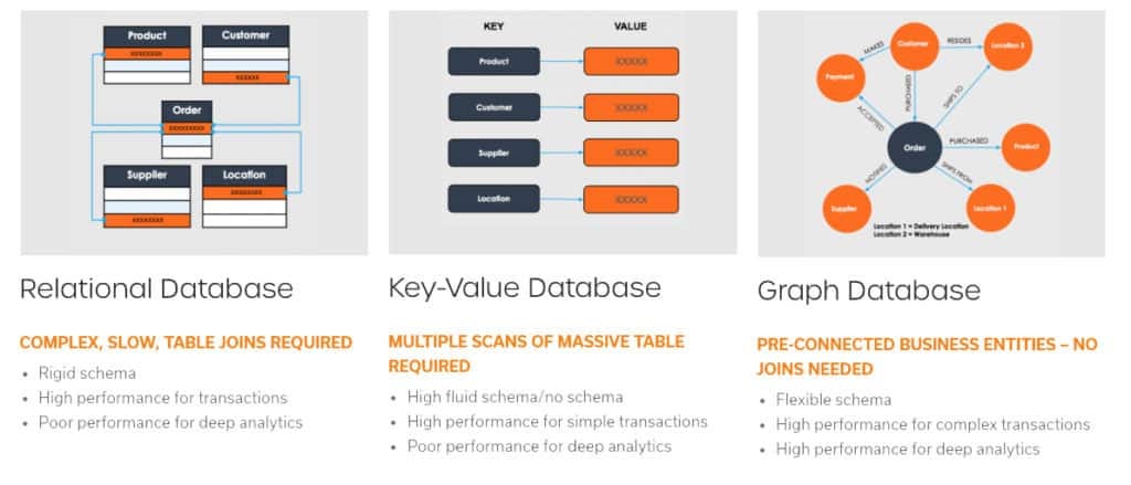
Pic credits : tigergraph
Indexes Indexes are very useful as they help speed up the query execution and helps faster retrieval of the data.
Syntax —
CREATE INDEX index_name
ON table (column_1, column_2, …column_n)
There are two types of indexes —
- Implicit indexes — indexes that are created by databases internally to store, retrieve faster and efficiently.
- Composite indexes — indexes that are created by using multiple columns to uniquely identify the data points.
Syntax —
CREATE UNIQUE INDEX index_name
ON tableName (column1, column2, …)
Example —
CREATE INDEX emp_indx
ON employee(emp_name, salary, city)
To drop the indexes —
ALTER TABLE table
DROP INDEX index_name
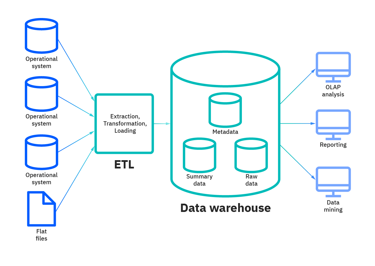
Pic credits : IBM
- Row oriented Storage — Most transactional databases use row oriented storage. The database is partitioned horizontally and with this approach writes are performed easily as compared to reads. Examples — PostgreSQL, MySQL and SQL Server. In row-oriented storage, data is stored as a series of rows, where each row represents a single record or tuple in the database. Each row contains all of the information for a particular record, including all of the attributes or columns. Row-oriented storage is optimized for fast retrieval of individual records, and it is a good choice for OLTP (Online Transaction Processing) systems that need to access individual records quickly.
Implementation of row-oriented storage using Python:
import sqlite3

# Create a connection to the database
conn = sqlite3.connect('example.db')# Create a cursor
cursor = conn.cursor()# Create a table
cursor.execute('CREATE TABLE users (id INTEGER PRIMARY KEY, name TEXT, email TEXT)')# Insert data into the table
cursor.execute("INSERT INTO users VALUES (1, 'John Doe', 'john.doe@example.com')")
cursor.execute("INSERT INTO users VALUES (2, 'Jane Smith', 'jane.smith@example.com')")# Retrieve data from the table
cursor.execute('SELECT * FROM users')
result = cursor.fetchall()print(result)
In this implementation, we use SQLite to create a row-oriented database. We create a table called “users” with three columns: id, name, and email. We insert two rows of data into the table and retrieve all rows from the table using a SELECT statement.
- Column oriented storage — In this every value is stored in the columns contiguously. The database is partitioned vertically and with this approach reads are performed easily as compared to writes. Examples — Redshift, BigQuery and Snowflake. In column-oriented storage, data is stored as a series of columns, where each column represents a single attribute or field in the database. Each column contains all of the values for a particular attribute, across all records in the database. Column-oriented storage is optimized for fast retrieval of large amounts of data for a specific attribute, and it is a good choice for OLAP (Online Analytical Processing) systems that need to perform aggregate calculations and data analysis.
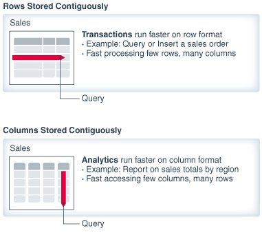
Pic credits : Oracle
Implementation of column-oriented storage using Python:
import pandas as pd

# Create a dataframe
data = {'id': [1, 2], 'name': ['John Doe', 'Jane Smith'], 'email': ['john.doe@example.com', 'jane.smith@example.com']}
df = pd.DataFrame(data)# Save the dataframe to a CSV file
df.to_csv('example.csv', index=False)# Load the data from the CSV file
df = pd.read_csv('example.csv')# Retrieve data from the dataframe
result = df[['id', 'name']]print(result)
In this implementation, we use Pandas to create a column-oriented database. We create a dataframe called “df” with three columns: id, name, and email. We save the dataframe to a CSV file and load the data from the CSV file. We retrieve the id and name columns from the dataframe using slicing.
- Data Cube — It allows data to be modeled and viewed in multiple dimensions. A data warehouse is based on a multidimensional data model which sees data in the form of a data cube. The data cube is constructed from a large, flat data set, such as a data warehouse, and it is organized into dimensions and measures. Dimensions represent the various aspects or attributes of the data, such as time, geography, or product. Measures represent the numeric values that describe the data, such as sales or profit.
- Each cell in the data cube represents a combination of dimension values and measure values, and it can be used to aggregate data in a flexible and efficient manner. For example, a data cube that stores sales information could have dimensions such as time, geography, and product, and measures such as sales and profit. Using the data cube, it would be possible to quickly retrieve and aggregate sales information by any combination of dimensions, such as sales by product, by region, or by quarter.
- The data cube structure is optimized for fast data analysis and aggregation, and it is especially useful for OLAP (Online Analytical Processing) systems that need to perform complex data analysis and reporting. The data cube supports fast data retrieval and aggregate calculations, such as sum, count, average, and so on, and it allows for the creation of reports and dashboards that provide insights into the data.
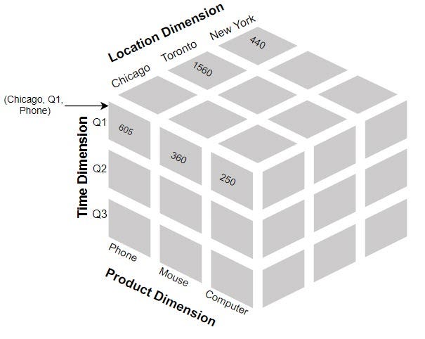
Pic credits : zineone
Implementation of a data cube using Python:
import numpy as np

# Create a 3-dimensional data cube
data_cube = np.array([
    [
        [1, 2, 3],
        [4, 5, 6],
        [7, 8, 9]
    ],
    [
        [10, 11, 12],
        [13, 14, 15],
        [16, 17, 18]
    ]
])# Query the data cube
result = data_cube[:, 0, 1]print(result)
In this implementation, we use NumPy to create a 3-dimensional data cube. The first dimension represents one attribute, the second dimension represents another attribute, and the third dimension represents a third attribute. We fill the data cube with sample data, and then query the data cube to retrieve the values at the first dimension index 0 and the second dimension index 1, which would be the values [2, 11] in this case. Data cubes can be used to efficiently store and query large datasets with multiple dimensions, such as sales data with dimensions for time, product, and location.
In conclusion, a data cube is a powerful tool for data analysis and aggregation in data warehousing and business intelligence applications. It provides a flexible and efficient way to store and retrieve data, and it enables fast and flexible data analysis and reporting.
It’s the process of translating objects into a format that can be stored in a file or memory buffer and transmitted across the network link and can be reconstructed later.
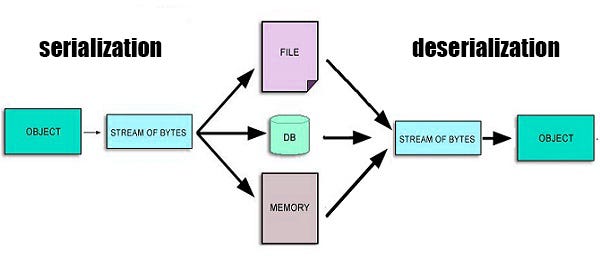
Pic credits : learninquizi
In serialization the objects are converted and stored within the computer memory into linear sequence of bytes which can be sent to another process/machine/file etc
Deserialization is the reverse of serialization in which the byte streams are converted into objects.
- Serialization refers to the process of converting an object or data structure into a sequence of bytes that can be stored or transmitted over a network. The process of serialization involves converting the object’s data into a binary or text format that can be written to disk or transmitted over a network. This enables the object to be easily stored, transmitted, and retrieved later.
- Deserialization is the inverse of serialization, and it involves converting a sequence of bytes back into the original object or data structure. The process of deserialization takes the serialized data, reads it from disk or receives it over a network, and converts it back into the original object.
One common way to serialize and deserialize data in a system is to use JSON (JavaScript Object Notation). JSON is a lightweight, text-based format that is easy to read and write for humans and machines alike.
Implementation of serialization and deserialization using Python’s built-in **json** module:
import json

# Create a Python dictionary to be serialized
data = {
    'name': 'John Smith',
    'age': 35,
    'interests': ['music', 'travel', 'photography']
}

# Serialize the dictionary to a JSON string
serialized_data = json.dumps(data)print(serialized_data)
# {"name": "John Smith", "age": 35, "interests": ["music", "travel", "photography"]}

# Deserialize the JSON string back into a Python dictionary
deserialized_data = json.loads(serialized_data)print(deserialized_data)
# {'name': 'John Smith', 'age': 35, 'interests': ['music', 'travel', 'photography']}
In this implementation, we start by creating a Python dictionary that we want to serialize. We then use the json.dumps() method to serialize the dictionary into a JSON-formatted string. We print the serialized data to the console to see the result. Next, we use the json.loads() method to deserialize the JSON-formatted string back into a Python dictionary. We print the deserialized data to the console to verify that it matches the original dictionary we created.
- Serialization and deserialization are widely used in a variety of applications, including data storage, remote procedure calls, and communication between different systems or services. For example, a web service might use serialization to convert data into a format that can be transmitted over the internet, and the client application might use deserialization to convert the data back into its original format for processing.
- When designing a system that uses serialization and deserialization, it is important to consider a number of factors, such as the format of the serialized data, the performance and scalability of the serialization and deserialization processes, and the compatibility of the serialized data between different systems. The choice of serialization format will depend on the specific requirements of the system, such as the size of the serialized data, the processing overhead of the serialization and deserialization processes, and the need for compatibility between different systems.
In conclusion, serialization and deserialization are important concepts in system design, and they play a critical role in data storage and communication between different systems. The choice of serialization format, the performance and scalability of the serialization and deserialization processes, and the compatibility of the serialized data between different systems are important considerations when designing a system that uses serialization and deserialization.
It is the process of creating replicas to store multiple copies of the same data on different machines ( may or may not be distributed geographically).
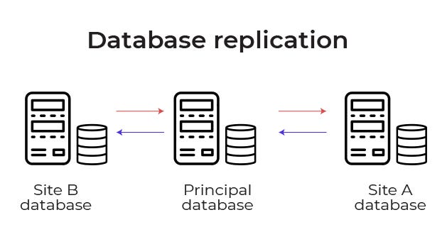
Pic credits : Databand
The most common types of replication include:
- Master-slave replication: In this type of replication, there is a designated master node that accepts all write operations, and one or more slave nodes that receive updates from the master node and serve read operations. This type of replication provides good performance for read operations, since the load can be distributed across multiple slave nodes, but it has a single point of failure in the master node.
Implementation of master-slave replication using MySQL:
-- Create a table in the master database
CREATE TABLE users (
    id INT PRIMARY KEY,
    name VARCHAR(50),
    email VARCHAR(50)
);

-- Create a slave database and configure replication
CHANGE MASTER TO
    MASTER_HOST='master-db.example.com',
    MASTER_USER='replication_user',
    MASTER_PASSWORD='replication_password',
    MASTER_LOG_FILE='mysql-bin.000001',
    MASTER_LOG_POS=100;-- Start replication
START SLAVE;
In this implementation, we first create a table in the master database. We then create a slave database and configure it to replicate data from the master database. We specify the host, user, password, and log file position to use for replication. Finally, we start the replication process.
2. Peer-to-peer replication: In this type of replication, all nodes are equal, and each node can accept both read and write operations. In this type of replication, there are no single points of failure, but the complexity of conflict resolution is increased, since multiple nodes may try to update the same data at the same time.
Implementation of peer-to-peer replication using PostgreSQL:
-- Create a table in each database
CREATE TABLE users (
    id INT PRIMARY KEY,
    name VARCHAR(50),
    email VARCHAR(50)
);

-- Configure replication for each database
ALTER SYSTEM SET synchronous_standby_names = 'node1,node2';-- Start replication
SELECT pg_create_logical_replication_slot('node1_slot', 'pgoutput');
SELECT pg_create_logical_replication_slot('node2_slot', 'pgoutput');
In this implementation, we create a table in each database that we want to replicate. We then configure replication for each database by setting the synchronous_standby_names parameter to the names of the other databases. Finally, we start replication by creating logical replication slots for each database.
3. Multi-master replication: This is similar to peer-to-peer replication, but it involves multiple master nodes that can accept write operations, and a mechanism for resolving conflicts that may arise between nodes.
Implementation of multi-master replication using MongoDB:
// Create a replica set with three nodes
rs.initiate({
    _id: 'myReplicaSet',
    members: [
        { _id: 0, host: 'node1.example.com:27017' },
        { _id: 1, host: 'node2.example.com:27017' },
        { _id: 2, host: 'node3.example.com:27017' }
    ]
});

// Enable multi-master replication
rs.conf().settings = { chainingAllowed: true };
rs.reconfig(rs.conf());
In this implementation, we first create a replica set with three nodes. We then enable multi-master replication by setting the chainingAllowed option to true and reconfiguring the replica set.
It helps in —
- Redundancy of the data
- Speeds up the process of reading and writing
- Reduces load on the databases
When designing a database system that uses replication, it is important to consider the trade-offs between performance, consistency, and availability, and to choose the type of replication that best fits the specific requirements of the system.
In conclusion, replication is a critical process in databases, and it is used to ensure data availability, reliability, and consistency across multiple nodes. There are several different types of replication, each with its own advantages and trade-offs, and the choice of replication type will depend on the specific requirements of the system.
In layman’s words, sharding is the technique to database partitioning that separates large and complex databases into smaller, faster and distributed databases for higher throughput operations.
To make databases —
1 . Faster and improve performance
2. Smaller and manageable
3. Reduce the transactional cost
4. Distributed and scale well
5. Speed up Query response time
6. Increases reliability and mitigates the after effects of outrages
Horizontal Sharding — divide the database table’s rows into multiple different tables where each part has the same schema and columns but different rows in order to create unique and independent partitions.
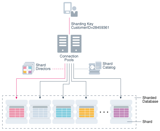
Pic credits: devcomm
Implementation of horizontal sharding in MongoDB:
// Connect to the MongoDB server
const MongoClient = require('mongodb').MongoClient;
const uri = "mongodb+srv://<username>:<password>@<cluster>.mongodb.net/test?retryWrites=true&w=majority";
const client = new MongoClient(uri, { useNewUrlParser: true });
client.connect(err => {
  if (err) throw err;
  const database = client.db("mydatabase");

  // Create a collection and shard it by a shard key
  database.createCollection("mycollection", {
    shardKey: { name: 1 }
  }, function(err, res) {
    if (err) throw err;
    console.log("Collection created!");
    client.close();
  });
});
In this implementation, we connect to a MongoDB server and create a collection called mycollection. We shard the collection by the_ name field using the shardKey option in the createCollection method.
Vertical Sharding — divide the database entire columns into new distinct tables such that each vertically partitioned parts are independent of all the others and have distinct rows and columns.
- Partitioning can be performed at the database level, or at the application level. When partitioning is performed at the database level, the database management system (DBMS) takes care of the partitioning and data distribution automatically. When partitioning is performed at the application level, the application must handle the partitioning and data distribution manually.
- When designing a system that uses partitioning, it is important to consider the trade-offs between scalability, performance, and consistency, and to choose the partitioning strategy that best fits the specific requirements of the system. In addition, it is important to consider the impact of partitioning on the overall system architecture and to design the system to accommodate the added complexity that partitioning introduces.
Implementation of vertical sharding in PostgreSQL:
-- Create a table and shard it by columns
CREATE TABLE mytable (
    id SERIAL PRIMARY KEY,
    name TEXT,
    email TEXT,
    age INTEGER,
    country TEXT
);

-- Create shards for each column
CREATE TABLE mytable_id (
    id SERIAL PRIMARY KEY,
    name TEXT
);
CREATE TABLE mytable_email (
    id SERIAL PRIMARY KEY,
    email TEXT
);
CREATE TABLE mytable_age (
    id SERIAL PRIMARY KEY,
    age INTEGER
);
CREATE TABLE mytable_country (
    id SERIAL PRIMARY KEY,
    country TEXT
);
In this implementation, we create a table called mytable with four columns. We then shard the table by creating separate tables for each column, with each table storing the column data and an ID column referencing the corresponding row in the original table.
In conclusion, partitioning, also known as sharding, is a technique used in databases to improve scalability and performance by dividing a large database into smaller, more manageable parts.
There are two main types of partitioning: horizontal partitioning and vertical partitioning, and the choice of partitioning strategy will depend on the specific requirements of the system.
When designing a system that uses partitioning, it is important to consider the trade-offs between scalability, performance, and consistency, and to design the system to accommodate the added complexity that partitioning introduces.
It’s a unit of program execution that accesses and updates the data items to preserve the integrity of the data that the DBMS should ensure using ACID properties.
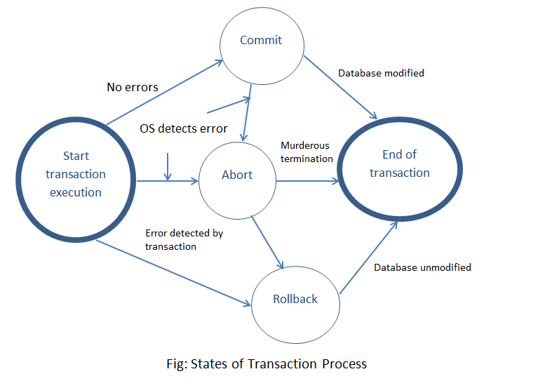
Pic credits : webduck
ACID means —
- Atomicity — It means either all the operations of a transaction are properly reflected in the database or none of them.
Implementation of an atomic transaction in PostgreSQL:
BEGIN;
UPDATE accounts SET balance = balance - 100 WHERE id = 123;
UPDATE accounts SET balance = balance + 100 WHERE id = 456;
COMMIT;
In this implementation, we begin a transaction using the BEGIN statement, and then update two rows in the accounts table. If either of these updates fails, the entire transaction will be rolled back using the ROLLBACK statement.
- Consistency- It means the execution of a transaction should be isolated so that data consistency be maintained.
Implementation of a consistent transaction in MySQL:
START TRANSACTION;
INSERT INTO orders (order_id, customer_id, order_total)
VALUES (1234, 5678, 100.00);
UPDATE customers SET balance = balance - 100.00 WHERE customer_id = 5678;
COMMIT;
In this implementation, we begin a transaction using the START TRANSACTION statement, and then insert a new order into the orders table. We also update the customers table to deduct the order total from the customer's balance. These changes satisfy the constraints defined by the database schema.
- Isolation — It means, in the situations where multiple transactions are executing, each transaction should be unaware of the other executing transaction and should be isolated.
Implementation of an isolated transaction in Oracle:
SET TRANSACTION ISOLATION LEVEL SERIALIZABLE;
BEGIN TRANSACTION;
UPDATE accounts SET balance = balance + 100 WHERE id = 123;
COMMIT TRANSACTION;
In this implementation, we set the isolation level of the transaction to SERIALIZABLE using the SET TRANSACTION statement, and then update the balance field for a single account in the accounts table. The database ensures that no other transactions are able to read or modify this row while the transaction is in progress.
- Durability- It means after the transaction is complete, the changes that are made to the database should persists even in case of system failures.
Implementation of a durable transaction in SQL Server:
BEGIN TRANSACTION;
UPDATE customers SET balance = balance - 100 WHERE customer_id = 123;
COMMIT TRANSACTION;
In this implementation, we begin a transaction using the BEGIN TRANSACTION statement, and then update the balance field for a single customer in the customers table. When we commit the transaction using the COMMIT TRANSACTION statement, the changes made to the database will be stored permanently and will be recoverable even in the event of system failures or crashes.
Transactions are atomic, meaning that they are indivisible and irreducible. This means that if a transaction is in progress, it will either be completed in full, or it will be rolled back to its original state, without leaving any intermediate states or partial changes.
- Transactions are also isolated, meaning that the operations within a transaction are isolated from other transactions and from any external changes to the database. This ensures that transactions are executed in a predictable and consistent manner, even if other transactions are executing concurrently.
- Transactions also have the property of durability, meaning that once a transaction has been committed, its changes are permanent and will survive any failures or other errors that may occur.
In a database, transactions are implemented by the database management system (DBMS) and are managed through a transaction manager. The transaction manager is responsible for coordinating the execution of transactions, enforcing the atomic, isolated, and durable properties of transactions, and providing a mechanism for managing any errors or failures that may occur during the execution of a transaction.
When designing a database system, it is important to consider the use of transactions and to ensure that the system is capable of supporting transactions in a way that meets the specific requirements of the system.
SQL and Databases : SQL is a programming language used to manage relational databases. SQL databases are used to store and retrieve data in a structured format and are commonly used in enterprise applications.
Implementation of a SQL database using MySQL:
CREATE TABLE customers (
  id INT PRIMARY KEY,
  name VARCHAR(50),
  email VARCHAR(50),
  phone VARCHAR(15)
);

CREATE TABLE orders (
  id INT PRIMARY KEY,
  customer_id INT,
  order_date DATE,
  total DECIMAL(10, 2),
  FOREIGN KEY (customer_id) REFERENCES customers(id)
);
In this implementation, we create two tables: customers and orders. The_ customers table has four columns: id,_ name,_ email, and_ phone. The_ id column is defined as the primary key, which means it uniquely identifies each row in the table. The orders table has four columns as well, with a foreign key constraint referencing the id column in the customers table.
Implementation of a NoSQL database using MongoDB:
db.createCollection("customers");

db.customers.insertOne({
  "_id": ObjectId("60ac737c3856b418bf6a0765"),
  "name": "John Doe",
  "email": "johndoe@example.com",
  "phone": "555-555-5555"
});db.createCollection("orders");db.orders.insertOne({
  "_id": ObjectId("60ac73b33856b418bf6a0766"),
  "customer_id": ObjectId("60ac737c3856b418bf6a0765"),
  "order_date": ISODate("2022-02-18T00:00:00Z"),
  "total": 100.00
});
In this implementation, we create two collections: customers and orders. The_ customers collection has a document with four fields: id,_ name,_ email, and_ phone. The_ id field is a unique identifier for the document, and is automatically generated by MongoDB when the document is inserted. The orders collection has a document with four fields as well, including a reference to the id field of a document in the customers collection.
Mongo DB : MongoDB is a NoSQL database that is designed for scalability and performance. It uses a document-based data model, which allows for flexible and dynamic schemas. MongoDB can be used for a wide range of applications, including big data, real-time analytics, and content management.
To connect to MongoDB from Python, you can use the PyMongo driver. You can install it using pip:
pip install pymongo
Connect to a local MongoDB instance:
from pymongo import MongoClient

# connect to MongoDB
client = MongoClient()# select database and collection
db = client['mydatabase']
collection = db['mycollection']To insert data into a MongoDB collection, you can use the insert_one() method:
# insert a document into the collection
document = {"name": "John Doe", "age": 30}
collection.insert_one(document)
You can also insert multiple documents at once using the insert_many() method:
# insert multiple documents into the collection
documents = [
    {"name": "Jane Doe", "age": 25},
    {"name": "Bob Smith", "age": 40},
    {"name": "Alice Brown", "age": 35},
]
collection.insert_many(documents)To query data from a MongoDB collection, you can use the find() method:
# find all documents in the collection
documents = collection.find()

# find documents that match a specific criteria
documents = collection.find({"age": {"$gte": 30}})
The find() method returns a cursor, which you can iterate over to access the individual documents. You can also use various modifiers and operators to refine your query.
To update data in a MongoDB collection, you can use the update_one() or update_many() method:
# update a single document in the collection
collection.update_one({"name": "John Doe"}, {"$set": {"age": 35}})

# update multiple documents in the collection
collection.update_many({"age": {"$lt": 30}}, {"$inc": {"age": 5}})
The update_one() method updates the first document that matches the query, while the update_many() method updates all documents that match the query.
To delete data from a MongoDB collection, you can use the `delete_one()` or `delete_many()` method:

# delete a single document from the collection
collection.delete_one({"name": "John Doe"})

# delete multiple documents from the collection
collection.delete_many({"age": {"$lt": 30}})
The delete_one() method deletes the first document that matches the query, while the delete_many() method deletes all documents that match the query.
Cassandra : Apache Cassandra is a NoSQL database that is designed to handle large amounts of data across many commodity servers, providing high availability with no single point of failure. Cassandra is a distributed, decentralized and highly-scalable database that is able to handle large amounts of data and provide high availability.
Connect to a local Cassandra cluster:
from cassandra.cluster import Cluster

# connect to Cassandra
cluster = Cluster()# create a session
session = cluster.connect()In Cassandra, a keyspace is a namespace that defines the replication strategy and other options for a set of tables. To create a keyspace, you can use the CREATE KEYSPACE statement:
# create a keyspace
session.execute("""
    CREATE KEYSPACE mykeyspace
    WITH replication = {'class': 'SimpleStrategy', 'replication_factor': '1'}
""")
This creates a keyspace with the name mykeyspace and a replication strategy of SimpleStrategy with a replication factor of 1.
In Cassandra, a table is defined by a set of columns and a primary key. To create a table, you can use the CREATE TABLE statement:
# create a table
session.execute("""
    CREATE TABLE mytable (
        id int PRIMARY KEY,
        name text,
        age int
    )
""")
This creates a table with the name mytable, with columns for id, name, and age. The id column is the primary key for the table.
To insert data into a Cassandra table, you can use the INSERT statement:
# insert data into the table
session.execute("""
    INSERT INTO mytable (id, name, age)
    VALUES (1, 'John Doe', 30)
""")
You can also insert multiple rows at once using the execute_batch() method:
# insert multiple rows into the table
rows = [
    (2, 'Jane Doe', 25),
    (3, 'Bob Smith', 40),
    (4, 'Alice Brown', 35),
]
query = "INSERT INTO mytable (id, name, age) VALUES (?, ?, ?)"
session.execute_batch(query, rows)To query data from a Cassandra table, you can use the SELECT statement:
# select all rows from the table
rows = session.execute("SELECT * FROM mytable")

# select rows that match a specific criteria
rows = session.execute("SELECT * FROM mytable WHERE age >= 30")
The execute() method returns a ResultSet, which you can iterate over to access the individual rows. You can also use various clauses and operators to refine your query.
To update data in a Cassandra table, you can use the UPDATE statement:
# update data in the table
session.execute("""
    UPDATE mytable SET age = 35 WHERE id = 1
""")
Pig: Pig is a high-level platform for creating MapReduce programs used with Hadoop. Pig allows for the creation of complex data pipelines using a simple SQL-like language called Pig Latin. Pig can also be used to process data on a single machine or a cluster of machines.
Implementation of a Pig Latin script:
Suppose we have a dataset with the following fields: user_id, age, gender, city, and state. We want to calculate the average age of users in each state. The Pig Latin script to accomplish this would be:
-- Load the data from the input file
`input_data = LOAD 'input_file.txt' USING PigStorage(',') AS (user_id:int, age:int, gender:chararray, city:chararray, state:chararray);
-- Group the data by state
grouped_data = GROUP input_data BY state;-- Calculate the average age for each group
average_age = FOREACH grouped_data GENERATE group AS state, AVG(input_data.age) AS avg_age;
-- Store the results in an output file
STORE average_age INTO 'output_file.txt' USING PigStorage(',');
In this script, we first load the data from the input file using the LOAD statement. We specify that the fields in the input file are comma-separated and define the schema of the input data using the AS statement. Next, we group the input data by state using the GROUP statement. This creates a set of groups, one for each unique state value. We then calculate the average age for each group using the AVG function in the FOREACH statement. This creates a new relation with two fields: state and avg_age. Finally, we store the results in an output file using the STORE statement. We specify that the fields in the output file should be comma-separated and use the USING statement to specify the output file format.
Hive: Hive is a data warehousing and SQL-like query language for Hadoop. It provides a way to organize and query large data sets stored in Hadoop Distributed File System (HDFS) and other storage systems.
Implementation of a Hive query:
Suppose we have a dataset with the following fields: user_id, age, gender, city, and state. We want to calculate the total number of male and female users in each state. The Hive query to accomplish this would be:
-- Create an external table to map to the input data
CREATE EXTERNAL TABLE users (user_id int, age int, gender string, city string, state string)
ROW FORMAT DELIMITED
FIELDS TERMINATED BY ','
LOCATION '/path/to/input/data';

-- Create a new table to store the results
CREATE TABLE user_counts (state string, male_count int, female_count int);-- Insert the results of the query into the new table
INSERT INTO user_counts
SELECT state,
       COUNT(CASE WHEN gender = 'M' THEN 1 END) AS male_count,
       COUNT(CASE WHEN gender = 'F' THEN 1 END) AS female_count
FROM users
GROUP BY state;
In this query, we first create an external table to map to the input data. We specify that the input data is delimited by commas and located in the HDFS file system. Next, we create a new table to store the results of the query. We define the schema of the table with three fields: state, male_count, and female_count. Finally, we insert the results of the query into the new table using the INSERT INTO statement. We use the SELECT statement to specify the query to execute. In this query, we use the CASE statement to count the number of male and female users in each state, and then group the results by state using the GROUP BY statement.
Spark: Apache Spark is an open-source, distributed computing system that is designed for big data processing. Spark provides an in-memory data processing engine that can run on top of Hadoop Distributed File System (HDFS), Amazon S3, and other storage systems. Spark can process data much faster than Hadoop MapReduce because it keeps data in memory.
Implementation of a Spark application using PySpark:
Suppose we have a dataset of customer orders with the following fields: order_id, customer_id, order_date, and order_amount. We want to calculate the total revenue generated from each customer in the dataset. The PySpark code to accomplish this would be:
from pyspark.sql import SparkSession
from pyspark.sql.functions import sum

# Create a SparkSession
spark = SparkSession.builder.appName("CustomerRevenue").getOrCreate()# Read the dataset into a DataFrame
orders = spark.read.format("csv").option("header", True).load("/path/to/orders")# Calculate the total revenue generated from each customer
customer_revenue = orders.groupBy("customer_id").agg(sum("order_amount").alias("total_revenue"))# Write the results to a file
customer_revenue.write.format("csv").option("header", True).mode("overwrite").save("/path/to/output")# Stop the SparkSession
spark.stop()
In this code, we first create a SparkSession, which is the entry point to programming Spark with the Dataset and DataFrame API. Next, we read the input data into a DataFrame using the read method and specify the format and location of the input file. We also specify that the input file has a header row. Then, we group the orders by customer_id using the groupBy method and aggregate the order amounts using the agg method and the sum function. We also give the resulting column a meaningful name using the alias method. Finally, we write the results to a file using the write method and specifying the format, location, and options for the output file. We also stop the SparkSession using the stop method.
Yarn: Yarn is a resource manager for Hadoop that allows for the allocation of resources such as CPU and memory to various applications running on a cluster. Yarn also manages the scheduling of tasks and the monitoring of their progress.
Implementation of YARN:
Suppose we have a Spark application that needs to be run on a YARN cluster. The following code can be used to submit the application:
$ spark-submit --master yarn \
               --deploy-mode cluster \
               --num-executors 10 \
               --executor-memory 4G \
               --executor-cores 4 \
               --driver-memory 2G \
               --class com.example.MyApp \
               myapp.jar
In this code, we use the spark-submit command-line tool to submit the Spark application. The --master option is set to yarn to indicate that the application should run on a YARN cluster. The --deploy-mode option is set to cluster to run the application in a distributed mode on the cluster. The --num-executors option specifies the number of executors to be used to run the application, while the --executor-memory option sets the amount of memory allocated to each executor. The --executor-cores option sets the number of cores allocated to each executor, while the --driver-memory option sets the amount of memory allocated to the driver program. Finally, the --class option specifies the fully-qualified class name of the main class of the application, and myapp.jar is the location of the JAR file containing the application code.
Hadoop: Hadoop is an open-source, distributed computing system that is designed for big data processing. It allows for the storage and processing of large data sets across a cluster of commodity servers. Hadoop includes the Hadoop Distributed File System (HDFS) for storage and the MapReduce programming model for processing.
Implementation of Hadoop:
Suppose we have a large file that needs to be processed using Hadoop. The following code can be used to upload the file to HDFS:
$ hdfs dfs -put /path/to/local/file /path/to/hdfs/directory/file
In this code, we use the hdfs dfs command to interact with HDFS. The -put option is used to upload a file from the local file system to HDFS. The first argument /path/to/local/file specifies the location of the file on the local file system, while the second argument /path/to/hdfs/directory/file specifies the location of the file in HDFS.
Once the file is uploaded to HDFS, we can process it using MapReduce. The following is an example implementation of MapReduce:
from mrjob.job import MRJob

class WordCount(MRJob):    def mapper(self, _, line):
        for word in line.split():
            yield word, 1    def reducer(self, word, counts):
        yield word, sum(counts)if __name__ == '__main__':
    WordCount.run()
In this code, we define a MapReduce job to count the occurrences of each word in the input file. The mapper function reads each line of the input file and emits each word with a count of 1. The reducer function receives the output of the mapper function, which consists of a list of values for each word, and sums the counts to obtain the total count for each word.
To run this job on Hadoop, we can use the following command:
$ python wordcount.py -r hadoop hdfs://<namenode>/path/to/input/file -o hdfs://<namenode>/path/to/output/directory
In this code, we use the mrjob library to define and run the MapReduce job. The -r option specifies the runner, which in this case is set to hadoop to indicate that the job should be run on Hadoop. The first argument hdfs:///path/to/input/file specifies the location of the input file in HDFS, while the second argument hdfs:///path/to/output/directory specifies the location of the output directory in HDFS.
Horizontal and vertical scaling refer to different methods of increasing a system’s capacity to handle increased load. Horizontal scaling involves adding more servers to a system, while vertical scaling involves adding more resources to a single server.
To implement horizontal scaling, we can add more instances of the application server and use a load balancer to distribute incoming requests across these instances.
Implementation using the Flask built-in development server:
from flask import Flask

app = Flask(__name__)@app.route("/")
def hello():
    return "Hello, World!"if __name__ == "__main__":
    app.run(debug=True, port=5000)
To run multiple instances of the server, we can use a process manager like gunicorn. Install_ gunicorn using pip:
pip install gunicorn
Then run the following command to start 4 instances of the server:
gunicorn --bind 0.0.0.0:5000 --workers 4 app:app
The --workers option specifies the number of worker processes to spawn, and the app:app argument tells gunicorn which Flask application object to use.
To implement vertical scaling, we can increase the resources (CPU, memory, disk space) of a single server.
Implementation using the Flask built-in development server:
from flask import Flask

app = Flask(__name__)@app.route("/")
def hello():
    return "Hello, World!"if __name__ == "__main__":
    app.run(debug=True, port=5000, threaded=True)
The threaded=True option tells Flask to run the server in multi-threaded mode, which can improve performance on multi-core systems.
Alternatively, we can use a production-ready server like gunicorn and specify the number of worker processes and threads per worker using the --workers and --threads options:
gunicorn --bind 0.0.0.0:5000 --workers 1 --threads 4 app:app
This starts a single worker process with 4 threads. Increasing the number of threads can improve performance by allowing multiple requests to be processed concurrently, but may also increase resource usage.
Load balancing and message queues are techniques used to distribute and manage workloads in a distributed system. Load balancing involves distributing incoming requests across multiple servers to ensure that no single server becomes overwhelmed, while message queues allow for asynchronous communication between different components of a system.
Implementation using Python Flask and the **Flask-LoadBalancer** extension:
from flask import Flask
from flask_loadbalancer import RoundRobinLoadBalancer

app = Flask(__name__)
lb = RoundRobinLoadBalancer(["http://server1:5000", "http://server2:5000", "http://server3:5000"])@app.route("/")
def hello():
    server = lb.next()
    response = requests.get(server)
    return response.contentif __name__ == "__main__":
    app.run(debug=True, port=5000)
The Flask-LoadBalancer extension provides a simple round-robin load balancing algorithm. We create a RoundRobinLoadBalancer object and pass in a list of server URLs. Then in our route handler, we use the load balancer to select the next server and send a request to it.
Message queues are used to decouple components of a distributed system by allowing them to communicate asynchronously.
Implementation using Python and the **pika** library:
import pika

# connect to RabbitMQ server
connection = pika.BlockingConnection(pika.ConnectionParameters(host='localhost'))
channel = connection.channel()# create a queue
channel.queue_declare(queue='task_queue', durable=True)def callback(ch, method, properties, body):
    print("Received message:", body)
    # do some work...
    print("Work done")
    ch.basic_ack(delivery_tag=method.delivery_tag)# set up a consumer to receive messages from the queue
channel.basic_qos(prefetch_count=1)
channel.basic_consume(queue='task_queue', on_message_callback=callback)# start consuming messages
print("Waiting for messages...")
channel.start_consuming()
We first connect to a RabbitMQ server and create a durable queue named task_queue. We then define a callback function to handle incoming messages, which in this example simply prints the message and then acknowledges it to remove it from the queue. Finally, we set up a consumer using the_ basic_consume method and start consuming messages using the start_consuming method.
To send messages to the queue, we can use the **basic_publish** method:
# connect to RabbitMQ server
connection = pika.BlockingConnection(pika.ConnectionParameters(host='localhost'))
channel = connection.channel()

# create a queue
channel.queue_declare(queue='task_queue', durable=True)# send a message
message = "Hello, world!"
channel.basic_publish(exchange='', routing_key='task_queue', body=message, properties=pika.BasicProperties(delivery_mode=2))
print("Sent message:", message)# close the connection
connection.close()
We first connect to the RabbitMQ server and declare the task_queue. Then we use the_ basic_publish method to send a message to the queue. The delivery_mode=2 option tells RabbitMQ to persist the message to disk so that it is not lost if the server crashes
High-level design and low-level design refer to different stages of the software development process. High-level design focuses on the overall architecture of a system and its major components, while low-level design focuses on the detailed design of individual components. Consistent Hashing is a technique used for distributed caching and load balancing.
Low-level design for the database component of a simple e-commerce website:
class Database:
    def __init__(self, db_name):
        self.db_name = db_name
        self.tables = {}

    def add_table(self, table_name, columns):
        self.tables[table_name] = Table(table_name, columns)    def get_table(self, table_name):
        return self.tables[table_name]class Table:
    def __init__(self, table_name, columns):
        self.table_name = table_name
        self.columns = columns
        self.rows = []    def insert_row(self, row):
        self.rows.append(row)    def get_rows(self):
        return self.rows
In this example, the Database class represents the overall database component of the system. It contains a dictionary of Table objects that represent individual tables within the database. The Table class represents an individual table within the database and contains a list of rows, where each row is represented as a dictionary of column values.
Monolithic and Microservices architecture are the two way of designing the software system. Monolithic is tightly coupled system where as Microservices is loosely coupled system.
Monolithic Architecture Implementation:
const express = require('express');
const app = express();app.get('/', (req, res) => {
  res.send('Hello World!');
});app.get('/users', (req, res) => {
  const users = [{ name: 'John Doe', age: 30 }, { name: 'Jane Smith', age: 25 }];
  res.send(users);
});app.listen(3000, () => {
  console.log('App listening on port 3000');
});
In the above implementation, the entire application is built and deployed as a single unit. It has two routes — “/” and “/users” — which return a simple “Hello World!” message and a list of users, respectively.
Microservices Architecture implementation:
const express = require('express');
const app = express();app.use(express.json());app.post('/login', (req, res) => {
  // authenticate user
  const user = { id: 1, name: 'John Doe' };
  res.send(user);
});app.listen(3000, () => {
  console.log('Auth service listening on port 3000');
});
const express = require('express');
const app = express();app.use(express.json());app.get('/users/:id', (req, res) => {
  // fetch user from database
  const user = { id: req.params.id, name: 'John Doe', age: 30 };
  res.send(user);
});app.listen(3001, () => {
  console.log('User service listening on port 3001');
});
In the above implementation, the application is divided into two services — an authentication service and a user service — each running on its own port. The authentication service handles user authentication and returns a user object upon successful authentication. The user service fetches user data from the database and returns it in response to a request to the “/users/:id” endpoint.
Caching, indexing, and proxies are techniques used to improve the performance of a system. Caching involves storing frequently-used data in memory for quick access, indexing involves creating an index of data to improve search performance, and proxies are used to forward requests to other servers or to cache responses.
Implementation of caching using Python and the LRU (Least Recently Used) algorithm:
import functools

@functools.lru_cache(maxsize=128)
def cached_function(x):
    # Function logic here
    return result
This code uses the functools.lru_cache() decorator to implement caching for a function. The maxsize parameter specifies the maximum number of cached items. The LRU algorithm ensures that the least recently used items are evicted from the cache when the maximum size is reached.
Implementation of indexing using SQL:
CREATE INDEX index_name
ON table_name (column_name);
This SQL code creates an index on a specified column in a table. This can significantly improve the performance of queries that involve that column.
Implementation of a proxy using Nginx:
http {
    server {
        listen 80;
        server_name example.com;
        location / {
            proxy_pass http://backend_server;
        }
    }
}
This Nginx configuration sets up a proxy server that listens for requests on port 80 for the domain example.com. All incoming requests are then passed to the backend server specified by the proxy_pass directive.
Networking, how browsers work, and content network delivery (CDN) are all related to the delivery of data over the internet. Networking involves the physical and logical connections between computers, browsers work by requesting and displaying web pages, and CDNs are a network of servers used to distribute content to users based on their geographic location.
Implementation of networking and CDN using Python:
import requests

# Networking example
response = requests.get('https://www.example.com')
print(response.text)# CDN example
from requests import Session
from requests.adapters import HTTPAdapter
from requests.packages.urllib3.util.retry import Retrysession = Session()
retry = Retry(total=5, backoff_factor=0.1, status_forcelist=[ 500, 502, 503, 504 ])
adapter = HTTPAdapter(max_retries=retry)
session.mount('http://', adapter)
session.mount('https://', adapter)response = session.get('https://cdn.example.com/image.jpg')
print(response.content)
In the above implementation, we use the Python requests library to make HTTP requests to a website and a CDN. The requests library handles the underlying network connections and provides a simple and consistent interface for working with web content. We also use the HTTPAdapter class to configure retries for failed requests, which can improve the reliability and robustness of our system.
Database sharding, CAP theorem, and database schema design are all related to the management of databases. Database sharding involves dividing a database into smaller, more manageable pieces, the CAP theorem is a principle that states that it is impossible for a distributed system to simultaneously provide consistency, availability, and partition tolerance, and database schema design involves creating a logical structure for storing data in a database.
Implement database sharding in Python using the PyMongo library:
from pymongo import MongoClient
from pymongo.errors import AutoReconnect

class Shard:
    def __init__(self, host, port):
        self.client = MongoClient(host, port)    def __getattr__(self, name):
        return getattr(self.client, name)    def __getitem__(self, key):
        return self.client[key]class ShardedMongoClient:
    def __init__(self, shards):
        self.shards = shards    def __getattr__(self, name):
        return getattr(self.shards[0], name)    def __getitem__(self, key):
        return self.shards[0][key]    def shard_key(self, key):
        return hash(key) % len(self.shards)    def shard_client(self, key):
        return self.shards[self.shard_key(key)]    def get(self, key):
        return self.shard_client(key).get(key)    def put(self, key, value):
        return self.shard_client(key).put(key, value)
In this implementation, we have two classes: Shard and ShardedMongoClient._ Shard represents a single shard of the database, while ShardedMongoClient represents the sharded database as a whole. The Shard class initializes a PyMongo client with the given host and port. The getattr and getitem methods are used to forward any method calls or attribute accesses to the underlying client object. The ShardedMongoClient class takes a list of Shard objects as input. The getattr and getitem methods are again used to forward method calls and attribute accesses to the appropriate shard. The shard_key method takes a key and returns an index into the list of shards. In this case, we're using a simple hash function to evenly distribute the keys among the shards. The shard_client method takes a key and returns the appropriate Shard object. This is used by the get and put methods to access the correct shard for a given key.
Implementation in Python of a distributed system that prioritizes availability and partition tolerance over consistency:
import random
from time import sleep

class DistributedSystem:
    def __init__(self, nodes):
        self.nodes = nodes    def put(self, key, value):
        for node in self.nodes:
            try:
                node.put(key, value)
            except NodeUnavailableError:
                continue
            else:
                return
        raise SystemUnavailableError("All nodes are unavailable")    def get(self, key):
        for node in self.nodes:
            try:
                return node.get(key)
            except NodeUnavailableError:
                continue
        raise SystemUnavailableError("All nodes are unavailable")class Node:
    def __init__(self, id, data=None):
        self.id = id
        self.data = data
        self.available = True    def put(self, key, value):
        if not self.available:
            raise NodeUnavailableError(f"Node {self.id} is currently unavailable")        # Introduce some artificial latency to simulate network delays
        sleep(random.uniform(0.1, 0.5))        self.data[key] = value    def get(self, key):
        if not self.available:
            raise NodeUnavailableError(f"Node {self.id} is currently unavailable")        # Introduce some artificial latency to simulate network delays
        sleep(random.uniform(0.1, 0.5))        return self.data.get(key)class NodeUnavailableError(Exception):
    passclass SystemUnavailableError(Exception):
    pass
In this implementation, the DistributedSystem class is the interface to the system, and it is responsible for deciding which node to send each request to. The put method sends a key-value pair to the distributed system, while the get method retrieves a value by key. The Node class represents an individual node in the distributed system. It has a unique ID, some data stored as a dictionary, and a flag indicating whether it is currently available. The put and get methods introduce some artificial latency to simulate network delays. If a node is unavailable (e.g., due to network partitioning), it will raise a NodeUnavailableError. If all nodes are unavailable, the_ DistributedSystem class will raise a SystemUnavailableError._
Concurrency, API, components, OOP, and abstraction are all related to the design and implementation of software. Concurrency involves executing multiple tasks simultaneously, API stands for Application Programming Interface which is the way for different systems to communicate with each other, Components are the building block of any system, OOP stands for Object Oriented Programming, and Abstraction is the process of hiding complexity and showing only the necessary details.
Implementing concurrency using Python’s threading module:
import threading

def task():
    print("Executing task...")# Create 10 threads
for i in range(10):
    t = threading.Thread(target=task)
    t.start()
Implementing an API using Python’s Flask framework:
from flask import Flask, request

app = Flask(__name__)@app.route('/hello', methods=['GET'])
def hello():
    name = request.args.get('name')
    return 'Hello, {}'.format(name)if __name__ == '__main__':
    app.run()
Implementing components using Python’s object-oriented programming:
class Car:
    def __init__(self, make, model, year):
        self.make = make
        self.model = model
        self.year = year

    def start(self):
        print("Starting the car...")
    def drive(self):
        print("Driving the car...")
my_car = Car('Toyota', 'Corolla', 2022)
my_car.start()
my_car.drive()
Implementing OOP using Python:
class Person:
    def __init__(self, name, age):
        self.name = name
        self.age = age
    def greet(self):
        print("Hello, my name is {} and I am {} years old.".format(self.name, self.age))person1 = Person("Alice", 25)
person1.greet()
person2 = Person("Bob", 30)
person2.greet()
Implementing abstraction using Python’s abstract base classes:
from abc import ABC, abstractmethod

class Animal(ABC):
    @abstractmethod
    def speak(self):
        passclass Dog(Animal):
    def speak(self):
        return "Woof!"class Cat(Animal):
    def speak(self):
        return "Meow!"class Duck(Animal):
    def speak(self):
        return "Quack!"animals = [Dog(), Cat(), Duck()]for animal in animals:
    print(animal.speak())
In this example, we define an abstract base class called Animal which has an abstract method called speak. This method is not implemented in the_ Animal class, but instead it's left to the subclasses to implement it. We then define three concrete subclasses of Animal:_ Dog,_ Cat, and_ Duck. Each of these classes implements the_ speak method in a different way. Finally, we create a list of Animal objects, which includes one instance of each subclass.
Estimation and planning, and performance are related to the management and evaluation of software systems. Estimation and planning involve determining the resources and time required to complete a project, while performance evaluation involves measuring and optimizing the performance of a system.
Implementation of a performance modeling technique called queueing theory using Python:
import math

def m_m_c_queue(lambda_, mu, c):
    rho = lambda_ / (c * mu)
    if rho >= 1:
        return None
    lq = ((c * rho)**c / (math.factorial(c) * (1 - rho))) * (rho / (1 - rho - (c * rho)**c / (math.factorial(c) * (1 - rho))))
    wq = lq / lambda_
    ls = lq + lambda_ / mu
    ws = ls / lambda_
    return (ls, ws, lq, wq)# Example usage
ls, ws, lq, wq = m_m_c_queue(10, 12, 3)
print(f"Average number of customers in the system: {ls}")
print(f"Average time a customer spends in the system: {ws}")
print(f"Average number of customers waiting in queue: {lq}")
print(f"Average time a customer spends waiting in queue: {wq}")
This code calculates the average number of customers in a queueing system with arrival rate lambda_, service rate_ mu, and_ c servers using the M/M/c queueing model. The output includes the average number of customers in the system (ls), the average time a customer spends in the system (ws), the average number of customers waiting in queue (lq), and the average time a customer spends waiting in queue (wq).
Performance can also be improved through techniques such as caching, indexing, and using proxies.
Implementation of caching using Python’s **functools** module:
import time
import functools

@functools.lru_cache(maxsize=None)
def expensive_function(x):
    time.sleep(1)
    return x * 2start_time = time.time()
result1 = expensive_function(10)
print(f"Result 1: {result1}")
print(f"Time taken: {time.time() - start_time}")start_time = time.time()
result2 = expensive_function(10)
print(f"Result 2: {result2}")
print(f"Time taken: {time.time() - start_time}")
This code defines a function expensive_function that takes a single argument x and returns x * 2 after waiting for 1 second to simulate an expensive computation. The @functools.lru_cache(maxsize=None) decorator enables caching of the function's results, so subsequent calls with the same argument will return the cached result without recomputing it. The maxsize=None argument means that the cache can store an unlimited number of results.
Map Reduce, patterns, and microservices are all related to the design and implementation of distributed systems. MapReduce is a programming model for processing large data sets, patterns are reusable solutions to common problems in software development, and microservices are a type of software architecture that involves building a system as a collection of small, independent services.
Implementation of word count in MapReduce using Python:
from mrjob.job import MRJob
import re

class MRWordCount(MRJob):    def mapper(self, _, line):
        words = re.findall(r'\w+', line)
        for word in words:
            yield word.lower(), 1    def reducer(self, word, counts):
        yield word, sum(counts)if __name__ == '__main__':
    MRWordCount.run()
In this implementation, the mapper function takes a line of text as input, splits it into individual words using a regular expression, and emits a key-value pair for each word with a count of 1. The reducer function receives these key-value pairs and sums the counts for each word, emitting the final count for each word.
Implementation of a simple microservice using Python:
from flask import Flask, jsonify

app = Flask(__name__)@app.route('/hello')
def hello():
    return jsonify({'message': 'Hello, world!'})if __name__ == '__main__':
    app.run()
In this implementation, we define a single route /hello that returns a JSON response with a "message" field containing the text "Hello, world!". The application is launched using the Flask web framework's built-in development server by calling app.run()._
SQL vs NoSQL, and cloud are all related to the management and storage of data. SQL (Structured Query Language) is a language used for managing relational databases, NoSQL databases are non-relational databases, and cloud refers to the delivery of computing services — including storage, databases, and software — over the internet.
Data & Data Flow: Refers to the movement of information from its source to its destination, involving various stages of processing and storage.
Implementation of a data flow system using Python:
import kafka
import json

# Set up Kafka producer
producer = kafka.KafkaProducer(bootstrap_servers='localhost:9092')# Define message to be sent
message = {'id': 1, 'name': 'John Doe', 'email': 'johndoe@example.com'}# Serialize message to JSON format
serialized_message = json.dumps(message).encode('utf-8')# Send message to Kafka topic
producer.send('my_topic', serialized_message)
In this implementation, we use the kafka library in Python to set up a Kafka producer and send a message to a topic called "my_topic". The message is first serialized to JSON format using the json library, then sent to the topic using the producer.send() method.
Databases types:
- SQL: Structured Query Language databases are relation databases that use tables and schema to store data.
- NoSQL: Non-Structured Query Language databases are a type of databases that do not follow the traditional relational model and can handle a variety of data types.
- Column: Column databases store data in columns, allowing for efficient queries on specific columns.
- Search: Search databases are specifically designed for text search and retrieval.
- Key Value: Key-value databases store data as key-value pairs, where the key is used to retrieve the value.
Anatomy of applications and services: Applications and services are composed of various components such as frontend, backend, databases, API, and message queues, among others.
Application Programming Interface (API): API is a set of protocols and routines for building software applications. It acts as a bridge between different applications and services, enabling communication and data exchange.
Implementing a simple API using Python and the Flask web framework:
from flask import Flask, request

app = Flask(__name__)# Define a simple endpoint that returns a greeting message
@app.route('/hello')
def hello():
    name = request.args.get('name', 'World')
    return f'Hello, {name}!'if __name__ == '__main__':
    app.run(debug=True)
In this implementation, we define a simple API with a single endpoint at /hello. When a user visits this endpoint, the_ hello() function is called and returns a greeting message using the name provided in the request parameters. We use the Flask web framework to define and run the API. The @app.route() decorator maps the /hello endpoint to the hello() function. The request object is used to access the request parameters, and the debug=True argument is passed to the app.run() method to enable debugging mode.
Caching: Caching refers to the temporary storage of data to speed up future requests.
Implement a simple cache for a function that calculates the nth Fibonacci number recursively :
import functools

@functools.lru_cache(maxsize=128)
def fibonacci(n):
    if n < 2:
        return n
    else:
        return fibonacci(n-1) + fibonacci(n-2)
In this implementation, we use the @functools.lru_cache(maxsize=128) decorator to specify that the results of the function should be cached using LRU (Least Recently Used) algorithm with a maximum cache size of 128. This means that if we call the fibonacci function with the same argument again, the result will be returned from the cache instead of re-calculating it.
REST API: Representational State Transfer API is a type of API that uses HTTP requests to GET, PUT, POST and DELETE data.
First, we will need to install the Flask module, which is a popular Python web framework for building REST APIs. We can do this by running the following command in our terminal:
pip install flask
Once we have installed Flask, we can create a simple REST API using the following code:
from flask import Flask, jsonify, request

app = Flask(__name__)# Define some sample data
products = [
    {'id': 1, 'name': 'Product 1'},
    {'id': 2, 'name': 'Product 2'},
    {'id': 3, 'name': 'Product 3'}
]# Define a route to get all products
@app.route('/products', methods=['GET'])
def get_products():
    return jsonify({'products': products})# Define a route to get a specific product
@app.route('/products/<int:id>', methods=['GET'])
def get_product(id):
    product = [p for p in products if p['id'] == id]
    if len(product) == 0:
        abort(404)
    return jsonify({'product': product[0]})# Define a route to create a new product
@app.route('/products', methods=['POST'])
def create_product():
    if not request.json or not 'name' in request.json:
        abort(400)
    product = {
        'id': products[-1]['id'] + 1,
        'name': request.json['name']
    }
    products.append(product)
    return jsonify({'product': product}), 201# Define a route to update a product
@app.route('/products/<int:id>', methods=['PUT'])
def update_product(id):
    product = [p for p in products if p['id'] == id]
    if len(product) == 0:
        abort(404)
    if not request.json:
        abort(400)
    if 'name' in request.json and type(request.json['name']) != str:
        abort(400)
    product[0]['name'] = request.json.get('name', product[0]['name'])
    return jsonify({'product': product[0]})# Define a route to delete a product
@app.route('/products/<int:id>', methods=['DELETE'])
def delete_product(id):
    product = [p for p in products if p['id'] == id]
    if len(product) == 0:
        abort(404)
    products.remove(product[0])
    return jsonify({'result': True})if __name__ == '__main__':
    app.run(debug=True)
In this code, we have created a Flask application and defined several routes to interact with a collection of products. We can run this application using the following command in our terminal:
python app.py
Once the application is running, we can use tools like Postman to interact with the REST API. For example, we can send a GET request to http://localhost:5000/products to retrieve all products, or a POST request to http://localhost:5000/products to create a new product. The API will return JSON data in response to each request.
Message Queues: Message Queues are systems that allow for asynchronous communication between applications, where messages are sent to a queue to be processed later.
Implement a simple message queue using Python and RabbitMQ as the message broker as follows —
- Install the pika library, which is a Python client for RabbitMQ.
pip install pika
- Create a connection to RabbitMQ and declare a queue.
import pika
connection = pika.BlockingConnection(
    pika.ConnectionParameters(host='localhost'))
channel = connection.channel()# declare a queue
channel.queue_declare(queue='my_queue')- Publish a message to the queue.
# publish a message to the queue
channel.basic_publish(exchange='', routing_key='my_queue', body='Hello, world!')- Consume messages from the queue.
# define a callback function to handle incoming messages
def callback(ch, method, properties, body):
    print("Received message:", body)

# start consuming messages from the queue
channel.basic_consume(queue='my_queue', on_message_callback=callback, auto_ack=True)
channel.start_consuming()
In this implementation, we first establish a connection to a RabbitMQ server running on localhost. We then declare a queue called “my_queue”. To publish a message to the queue, we call the basic_publish() method on the channel object. To consume messages from the queue, we define a callback function that handles incoming messages and pass it to the basic_consume() method along with the queue name. Finally, we start consuming messages by calling start_consuming()._
Pub-Sub Messaging: Publish-Subscribe messaging is a messaging pattern where publishers send messages to a queue, and subscribers receive and process the messages.
To implement Pub-Sub messaging, we can use a message broker that acts as an intermediary between publishers and subscribers.
Implementation using Python and the **paho-mqtt** library:
import paho.mqtt.client as mqtt

# Define callback functions for connection and message received events
def on_connect(client, userdata, flags, rc):
    print("Connected with result code " + str(rc))
    # Subscribe to topic on connection
    client.subscribe("test/topic")def on_message(client, userdata, msg):
    print(msg.topic + " " + str(msg.payload))# Create MQTT client instance and connect to broker
client = mqtt.Client()
client.on_connect = on_connect
client.on_message = on_message
client.connect("localhost", 1883, 60)# Start MQTT client loop to process incoming messages
client.loop_start()# Publish message to topic
client.publish("test/topic", "Hello, world!")# Stop MQTT client loop after publishing message
client.loop_stop()
In this example, we first define callback functions for the on_connect and on_message events that are triggered by the MQTT client. The on_connect function subscribes to the topic "test/topic" upon connecting to the broker. The on_message function simply prints the received message to the console. We then create an instance of the MQTT client and connect to a local broker. We start the client loop to continuously process incoming messages. Finally, we publish a message to the "test/topic" topic and stop the client loop after publishing the message.
Performance Metrics: Performance metrics are measures used to evaluate the efficiency and effectiveness of a software or system.
Implementation in Python to measure the performance metrics of a function:
import time

def my_function():
    time.sleep(1) # Simulate some time-consuming operation
    return "Hello World"start_time = time.time()
result = my_function()
end_time = time.time()response_time = end_time - start_time
print("Response time:", response_time)# Calculate throughput by calling the function multiple times
num_requests = 100
start_time = time.time()
for i in range(num_requests):
    result = my_function()
end_time = time.time()throughput = num_requests / (end_time - start_time)
print("Throughput:", throughput)# Measure latency
start_time = time.time()
result = my_function()
end_time = time.time()latency = end_time - start_time
print("Latency:", latency)# Measure CPU utilization
import psutil
cpu_utilization = psutil.cpu_percent()
print("CPU utilization:", cpu_utilization)# Measure memory usage
memory_usage = psutil.virtual_memory().percent
print("Memory usage:", memory_usage)# Measure disk I/O
disk_io = psutil.disk_io_counters().read_count
print("Disk I/O:", disk_io)# Measure network traffic
network_traffic = psutil.net_io_counters().bytes_sent + psutil.net_io_counters().bytes_recv
print("Network traffic:", network_traffic)
In this example, we first define a function my_function that simulates some time-consuming operation. We then measure the response time of the function by calculating the time taken between calling the function and receiving the result. We then measure the throughput of the function by calling it multiple times and dividing the number of requests by the total time taken. We also measure the latency of the function by calculating the time taken to receive the result from a single call. Next, we use the psutil library to measure the CPU utilization, memory usage, disk I/O, and network traffic of the system.
Fault and Failure in Distributed Systems: Fault refers to a defect or error in a system, while failure refers to the inability of a system to perform its intended function. In distributed systems, faults and failures can occur due to network partitions, node crashes, and other reasons.
The Raft consensus algorithm is a widely used algorithm for achieving fault tolerance in distributed systems. Here’s an example implementation of a fault-tolerant distributed system using Python and the Raft consensus algorithm:
First, let’s define a simple key-value store that we want to make fault-tolerant:
class KeyValueStore:
    def __init__(self):
        self.store = {}

    def get(self, key):
        return self.store.get(key)    def set(self, key, value):
        self.store[key] = value
Now, let’s define the Raft consensus algorithm. We’ll start with the Node class, which represents a node in the cluster:
from enum import Enum

class NodeState(Enum):
    FOLLOWER = 0
    CANDIDATE = 1
    LEADER = 2class Node:
    def __init__(self, id, cluster):
        self.id = id
        self.cluster = cluster
        self.state = NodeState.FOLLOWER
        self.current_term = 0
        self.voted_for = None
        self.log = []
        self.commit_index = 0
        self.last_applied = 0
        self.next_index = {}
        self.match_index = {}
    def request_vote(self, candidate_id, last_log_index, last_log_term):
        pass
    def append_entries(self, leader_id, prev_log_index, prev_log_term, entries, leader_commit):
        pass
    def start_election(self):
        pass
    def send_heartbeat(self):
        pass
The Node class has several instance variables that store the node's current state, as well as its log and commit index. It also has methods for handling requests for votes and append entries, as well as starting an election and sending heartbeats.
Next, we’ll define the Cluster class, which represents the entire cluster of nodes:
class Cluster:
    def __init__(self, nodes):
        self.nodes = nodes
        self.leader = None

    def request_vote(self, candidate_id, last_log_index, last_log_term):
        pass
    def append_entries(self, leader_id, prev_log_index, prev_log_term, entries, leader_commit):
        pass
    def start_election(self):
        pass
    def send_heartbeats(self):
        pass
The Cluster class has methods for handling requests for votes and append entries, as well as starting an election and sending heartbeats.
Finally, let’s put everything together and define the main function that runs the cluster:
import time

class Raft:
    def __init__(self, cluster):
        self.cluster = cluster    def run(self):
        while True:
            time.sleep(1)
            self.cluster.send_heartbeats()if __name__ == '__main__':
    nodes = [Node(0, None), Node(1, None), Node(2, None)]
    cluster = Cluster(nodes)
    raft = Raft(cluster)
    raft.run()
This code creates a cluster of three nodes and runs the Raft object, which simply sends heartbeats every second.
Horizontal vs Vertical Scaling: Horizontal scaling involves adding more nodes to a system to increase its capacity, while vertical scaling involves adding more resources to a single node.
Horizontal Scaling
Let’s say we have a simple web application that uses a Flask framework to serve HTTP requests. To horizontally scale this application, we can use a load balancer to distribute traffic among multiple instances of the application running on different servers.
Implementation of a simple load balancer using Flask:
from flask import Flask
from werkzeug.contrib.fixers import ProxyFix

app = Flask(__name__)@app.route("/")
def hello():
    return "Hello, World!"if __name__ == "__main__":
    app.wsgi_app = ProxyFix(app.wsgi_app)
    app.run(port=5000)
To horizontally scale this application, we can use a load balancer like Nginx to distribute traffic among multiple instances of this application running on different servers. Here’s an implementation Nginx configuration file:
http {
    upstream my_app {
        server 10.0.0.1:5000;
        server 10.0.0.2:5000;
        server 10.0.0.3:5000;
    }

    server {
        listen 80;
        location / {
            proxy_pass [http://my_app;](http://my_app;)
            proxy_set_header Host $host;
            proxy_set_header X-Real-IP $remote_addr;
            proxy_set_header X-Forwarded-For $proxy_add_x_forwarded_for;
        }
    }
}
This configuration tells Nginx to distribute traffic among three instances of the application running on three different servers with IP addresses 10.0.0.1, 10.0.0.2, and 10.0.0.3.
Vertical scaling involves adding more resources to an existing server to handle increased traffic and data processing. This can include adding more CPU, RAM, and storage to the server.
Implementation of increasing the RAM of a server using Python:
import psutil

# Get the current memory usage of the server
mem = psutil.virtual_memory()# Print the current memory usage
print(f"Current Memory Usage: {mem.used} bytes")# Increase the memory by 2 GB
new_mem = mem.total + 2 * 1024 * 1024 * 1024# Set the new memory value
psutil.virtual_memory().total = new_mem# Print the new memory value
print(f"New Memory Value: {new_mem} bytes")
In this example, we first import the psutil library, which allows us to access system resources such as CPU, memory, and disk usage. We then get the current memory usage of the server using the psutil.virtual_memory() method and print it to the console. Next, we increase the memory of the server by 2 GB by adding 2 * 1024 * 1024 * 1024 to the current memory value. We then set the new memory value using the psutil.virtual_memory().total property and print the new memory value to the console.
Database Replication: Database replication is the process of copying data from one database to another to ensure data consistency and availability.
Python code for starting the replication process:
import mysql.connector

# Define the database configuration parameters
config = {
    'user': 'replication_user',
    'password': 'replication_password',
    'host': 'primary_server_ip',
    'database': 'database_name',
    'charset': 'utf8mb4',
    'use_unicode': True,
}# Connect to the primary server
conn = mysql.connector.connect(**config)# Start the replication process
cursor = conn.cursor()
cursor.execute("STOP SLAVE;")
cursor.execute("CHANGE MASTER TO MASTER_HOST='primary_server_ip', \
                MASTER_USER='replication_user', MASTER_PASSWORD='replication_password', \
                MASTER_LOG_FILE='mysql-bin.000001', MASTER_LOG_POS= 107;")  # set the appropriate log file and position
cursor.execute("START SLAVE;")
cursor.close()
conn.close()# Monitor the replication status
conn = mysql.connector.connect(user='replication_user', password='replication_password',
                               host='secondary_server_ip', database='database_name')
cursor = conn.cursor()
cursor.execute("SHOW SLAVE STATUS;")
result = cursor.fetchone()
if result[10] == 'Yes':  # check if the replication is running
    print('Replication is running')
else:
    print('Replication is not running')
cursor.close()
conn.close()
This code connects to the primary server and starts the replication process using the CHANGE MASTER TO SQL statement. It then checks the replication status using the SHOW SLAVE STATUS SQL statement and prints the status to the console. Note that you need to replace the configuration parameters with the appropriate values for your system.
CAP Theorem: CAP theorem states that a distributed system cannot simultaneously provide Consistency, Availability, and Partition tolerance.
Implementation of a distributed key-value store that demonstrates the CAP theorem:
import java.util.HashMap;

public class DistributedKeyValueStore {
    private HashMap<String, String> data;
    private boolean isAvailable;
    private boolean isConsistent;
    private boolean isPartitionTolerant;    public DistributedKeyValueStore() {
        data = new HashMap<>();
        isAvailable = true;
        isConsistent = true;
        isPartitionTolerant = true;
    }    public String get(String key) {
        if (!isAvailable) {
            throw new RuntimeException("System is unavailable.");
        }        if (!isPartitionTolerant) {
            throw new RuntimeException("System is not partition tolerant.");
        }        return data.get(key);
    }    public void put(String key, String value) {
        if (!isAvailable) {
            throw new RuntimeException("System is unavailable.");
        }        if (!isPartitionTolerant) {
            throw new RuntimeException("System is not partition tolerant.");
        }        if (!isConsistent) {
            // Perform eventual consistency
            // ...            // Update data with new value
            data.put(key, value);
        } else {
            // Update data with new value
            data.put(key, value);
        }
    }    public void setAvailability(boolean isAvailable) {
        this.isAvailable = isAvailable;
    }    public void setConsistency(boolean isConsistent) {
        this.isConsistent = isConsistent;
    }    public void setPartitionTolerance(boolean isPartitionTolerant) {
        this.isPartitionTolerant = isPartitionTolerant;
    }
}
In this implementation, the DistributedKeyValueStore class represents a distributed key-value store. The get and put methods provide the basic operations to retrieve and store data. The isAvailable,_ isConsistent, and_ isPartitionTolerant boolean variables represent the state of the system with respect to each of the three guarantees of the CAP theorem. The setAvailability,_ setConsistency, and_ setPartitionTolerance methods allow the system's state to be changed at runtime.
In order to enforce the guarantees of the CAP theorem, the get and put methods check the state of the system before performing any operations. If the system is not available or not partition tolerant, an exception is thrown. If the system is consistent, the put method updates the data immediately. If the system is not consistent, the put method performs eventual consistency before updating the data.
Database Sharding: Database sharding is the process of splitting a database into smaller, more manageable parts called shards.
Implement sharding logic in a Node.js application using a middleware layer:
const express = require('express');
const app = express();

// Middleware to intercept queries and send them to the correct shard
app.use((req, res, next) => {
  const userId = req.query.userId; // Assume sharding by user ID
  const shardId = getShardId(userId); // Determine which shard to use
  const shardUrl = getShardUrl(shardId); // Determine URL for shard  // Send query to appropriate shard
  axios.get(`${shardUrl}/query`, { params: req.query })
    .then(response => res.send(response.data))
    .catch(error => next(error));
});// Function to determine shard ID based on user ID
function getShardId(userId) {
  // Determine shard ID based on user ID
  // ...
}// Function to determine shard URL based on shard ID
function getShardUrl(shardId) {
  // Determine URL for shard based on shard ID
  // ...
}app.listen(3000, () => console.log('Server started on port 3000'));
This code assumes that each shard has a unique URL that can be used to send queries to that shard. The getShardId function determines the shard ID based on the user ID, and the getShardUrl function determines the URL for the shard based on the shard ID. The middleware layer intercepts queries and sends them to the appropriate shard using the axios library.
Consistent Hashing: Consistent Hashing is a method of distributing data across multiple nodes in a way that minimizes remapping when nodes are added or removed.
Implement consistent hashing in a Node.js application:
const crypto = require('crypto');

// Class representing a node in the hash ring
class Node {
  constructor(id) {
    this.id = id;
    this.virtualNodes = [];
  }
}// Class representing a consistent hash ring
class HashRing {
  constructor(nodes, numVirtualNodes, hashFn) {
    this.nodes = nodes;
    this.numVirtualNodes = numVirtualNodes;
    this.hashFn = hashFn;
    this.virtualNodes = [];    // Initialize virtual nodes for each node
    for (let i = 0; i < nodes.length; i++) {
      for (let j = 0; j < numVirtualNodes; j++) {
        const virtualNodeId = `${nodes[i].id}-vnode-${j}`;
        const virtualNodeHash = this.hashFn(virtualNodeId);
        this.virtualNodes.push({ hash: virtualNodeHash, node: nodes[i] });
        nodes[i].virtualNodes.push(virtualNodeHash);
      }
    }
    // Sort virtual nodes in hash ring order
    this.virtualNodes.sort((a, b) => a.hash - b.hash);
  }  // Method to find the node responsible for a given key
  getNodeForKey(key) {
    const keyHash = this.hashFn(key);
    const virtualNode = this.findNextVirtualNode(keyHash);
    return virtualNode.node;
  }  // Method to find the next virtual node in the hash ring
  findNextVirtualNode(hash) {
    for (let i = 0; i < this.virtualNodes.length; i++) {
      if (hash <= this.virtualNodes[i].hash) {
        return this.virtualNodes[i];
      }
    }
    return this.virtualNodes[0];
  }
}
// Example usage
const nodes = [new Node('node1'), new Node('node2'), new Node('node3')];
const hashRing = new HashRing(nodes, 100, key => {
  const hash = crypto.createHash('sha1');
  hash.update(key);
  return parseInt(hash.digest('hex').slice(0, 8), 16);
});// Map keys to nodes
const key1 = 'foo';
const key2 = 'bar';
const node1 = hashRing.getNodeForKey(key1);
const node2 = hashRing.getNodeForKey(key2);
console.log(`Node for ${key1}: ${node1.id}`);
console.log(`Node for ${key2}: ${node2.id}`);// Handle node failures
nodes.splice(1, 1); // remove node2
hashRing.nodes = nodes;
hashRing.virtualNodes = [];
hashRing.virtualNodes = hashRing.virtualNodes.concat(nodes.reduce((acc, node) => acc.concat(node.virtualNodes), []));
hashRing.virtualNodes.sort((a, b) => a.hash - b.hash);
const node3 = hashRing.getNodeForKey(key1);
const node4 = hashRing.getNodeForKey(key2);
console.log(`Node for ${key1}: ${node3.id}`);
console.log(`Node for ${key2}: ${node4.id}`);
In this example, we first create three nodes and a hash ring with 100 virtual nodes using the SHA-1 hashing algorithm. We then map two keys to nodes using the getNodeForKey method, and print out the nodes that are responsible for each key. Next, we simulate a node failure by removing node2 from the list of nodes. We update the nodes array in the hash ring and regenerate the virtual nodes to account for the missing node.
A Distributed Message Queue (DMQ) is a distributed system component that enables asynchronous communication and decoupling between various components in a distributed system. It provides a reliable and scalable way to exchange messages between producers and consumers, ensuring reliable delivery and efficient processing of messages. DMQs act as intermediaries, allowing producers to send messages to a queue and consumers to receive and process those messages at their own pace.
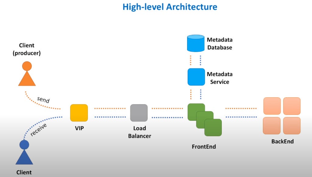
PIC CREDITS: STACKOVERFLOW
Key features and benefits of using DMQs in distributed systems:
- Asynchronous communication: DMQs enable decoupling between components by allowing them to communicate asynchronously. Producers can send messages without waiting for immediate responses, and consumers can process messages independently of the producers.
- Scalability and flexibility: DMQs can handle high message throughput and scale horizontally by adding more brokers or queue instances. They provide a flexible and elastic messaging infrastructure that can adapt to changing workloads.
- Fault tolerance and reliability: DMQs ensure reliable message delivery by providing mechanisms for message persistence, replication, and fault tolerance. They can recover from failures and continue message processing without data loss.
- Load balancing and distribution: DMQs distribute messages across multiple brokers or queue instances, allowing for load balancing and parallel processing of messages. This improves system performance and resource utilization.
- Message durability: DMQs store messages in a durable manner, ensuring that messages are not lost even in the event of system failures or restarts. This guarantees reliable message processing and prevents data loss.
Common use cases and scenarios where DMQs are applicable: DMQs are widely used in various distributed systems scenarios, including:
- Event-driven architectures: DMQs enable the building of event-driven systems where components react to events by producing or consuming messages. This approach allows for loose coupling, scalability, and extensibility.
- Microservices communication: DMQs facilitate communication between microservices by providing an asynchronous and decoupled messaging mechanism. They enable microservices to communicate without relying on synchronous request-response patterns, improving overall system performance and resilience.
- Stream processing and data pipelines: DMQs can be used as the backbone for building scalable and fault-tolerant stream processing systems. They allow for the ingestion, processing, and delivery of high-volume streaming data while ensuring reliability and fault tolerance.
- Task distribution and workload balancing: DMQs can distribute tasks or workload across multiple consumers, enabling parallel processing and load balancing. This is particularly useful in scenarios where tasks can be processed independently and in parallel.
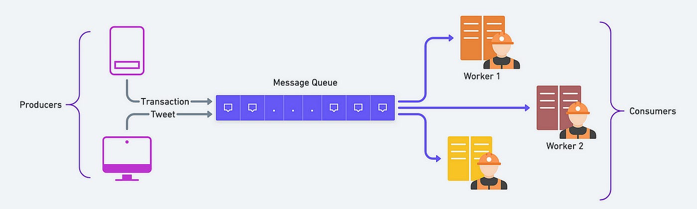
Pic credits : Devgenius
Overview of the architecture and components of a DMQ system: A typical DMQ system consists of the following main components:
- Producers: Producers are responsible for generating and sending messages to the DMQ system. They publish messages to a specific queue or topic for further processing by consumers.
- Consumers: Consumers are components that subscribe to queues or topics and receive messages from the DMQ system. They process and act upon the received messages according to the application logic.
- Brokers: Brokers are the core components of a DMQ system. They receive messages from producers, store them temporarily, and deliver them to the appropriate consumers. Brokers handle message routing, queuing, and load balancing.
- Queues: Queues are data structures within the DMQ system that hold the messages sent by producers until they are consumed by consumers. They provide the storage and buffering mechanism for messages.
How messages are routed and stored within the DMQ system: When a producer sends a message, it is typically directed to a specific queue or topic. The broker responsible for that queue receives the message and stores it temporarily. The message is then made available to interested consumers subscribed to that queue or topic.
Role of metadata and how it is managed within the system: Metadata plays a crucial role in a DMQ system as it provides essential information about messages, queues, and system configuration. It includes details such as message headers, routing information, message priority, timestamps, and consumer subscription information. Metadata helps in routing messages to the appropriate queues, ensuring message delivery guarantees, and managing system resources efficiently.
The DMQ system manages metadata through various mechanisms, including:
- Message headers: Each message typically contains headers that carry metadata about the message, such as the message ID, timestamp, and other application-specific properties. These headers are used by the DMQ system to route and process messages.
- Queue metadata: The DMQ system maintains metadata related to queues, such as their names, capacities, and access control policies. This information allows the system to efficiently manage message storage, routing, and consumer subscriptions.
- Consumer subscription metadata: The system keeps track of consumer subscriptions to queues or topics. This metadata includes information about which consumers are interested in specific queues or topics, enabling the system to deliver messages to the appropriate consumers.
Communication Protocols and Messaging Models:
DMQ systems support various communication protocols, each with its own characteristics and use cases. Some commonly used protocols include:
- Advanced Message Queuing Protocol (AMQP): AMQP is an open standard protocol for message-oriented middleware. It provides a reliable, secure, and interoperable messaging solution with features such as message queuing, routing, and transaction support.
- Message Queuing Telemetry Transport (MQTT): MQTT is a lightweight publish-subscribe messaging protocol designed for resource-constrained devices and low-bandwidth networks. It is commonly used in IoT scenarios where devices need to exchange messages efficiently.
- Kafka Protocol: Kafka Protocol is the communication protocol used by Apache Kafka, a distributed streaming platform. It is designed for high-throughput, fault-tolerant, and scalable event streaming applications.
DMQs support different messaging models to cater to various application requirements. Some common messaging models include:
- Publish-Subscribe: In the publish-subscribe model, messages are published to topics, and multiple consumers can subscribe to receive messages from those topics. This model allows for one-to-many communication and is suitable for scenarios where messages need to be broadcasted to multiple consumers.
- Point-to-Point: In the point-to-point model, messages are sent to specific queues, and only one consumer receives and processes each message. This model ensures that each message is consumed by exactly one consumer and is suitable for scenarios where workload distribution or task processing is required.
- Request-Reply: The request-reply model involves a two-way communication pattern where a client sends a request message, and a server responds with a reply message. This model is useful for synchronous interactions and RPC-style communication.
Pros and cons of each messaging model and considerations for choosing the appropriate model for different use cases:
- Publish-Subscribe:
- Pros: Enables broadcast-style messaging, supports decoupled communication, and allows for dynamic scaling of consumers. It is suitable for scenarios where multiple consumers need to receive the same message or where there is a need for event-driven architectures.
- Cons: Can introduce additional complexity in ensuring message ordering and consistency across subscribers.
- Point-to-Point:
- Pros: Ensures each message is consumed by a single consumer, simplifies message ordering, and allows for workload distribution. It is suitable for scenarios where task processing needs to be distributed among multiple consumers and message order is important.
- Cons: May not scale well when there are a large number of consumers competing for messages from a single queue.
- Request-Reply:
- Pros: Supports synchronous communication patterns, supports request-response interactions, and enables real-time communication between clients and servers. It is suitable for scenarios where immediate responses are required.
- Cons: May introduce tight coupling between clients and servers, can result in increased latency due to synchronous nature, and may require additional coordination mechanisms for load balancing and fault tolerance.
- When choosing the appropriate messaging model for different use cases, considerations include the nature of the communication (one-to-many or one-to-one), message ordering requirements, scalability requirements, latency sensitivity, and the need for synchronous or asynchronous communication.
Scalability and High Availability:
- Techniques and strategies for scaling DMQ systems to handle high message throughput: To scale DMQ systems and handle high message throughput, the following techniques and strategies can be employed:
- Horizontal scaling: DMQ systems can be horizontally scaled by adding more broker instances to distribute the message processing load. Load balancers can be used to distribute incoming messages across multiple brokers, ensuring efficient utilization of resources.
- Partitioning: Partitioning or sharding involves dividing the message queues into smaller partitions and distributing them across multiple brokers. Each partition can be independently processed, allowing for parallel processing and improved scalability.
- Clustering: Clustering involves creating a cluster of brokers that work together as a single logical unit. This provides fault tolerance, high availability, and load balancing across the brokers in the cluster.
Load balancing and partitioning approaches to distribute messages across multiple brokers: To distribute messages across multiple brokers in a DMQ system, load balancing and partitioning approaches are used:
- Round-robin load balancing: Messages are evenly distributed among brokers in a round-robin fashion. Each incoming message is routed to the next available broker in a cyclic manner, ensuring balanced utilization of resources.
- Hash-based partitioning: Messages are assigned to partitions based on a hash function applied to a message attribute or key. The hash value determines the target partition, and each broker is responsible for processing specific partitions.
- Consistent hashing: Consistent hashing ensures minimal disruption when the number of brokers changes. It uses a hash function to map both messages and brokers to a common identifier space, allowing efficient load balancing and reassignment of partitions during dynamic scaling.
Replication and data redundancy mechanisms to ensure high availability and fault tolerance: To ensure high availability and fault tolerance in DMQ systems, replication and data redundancy mechanisms are employed:
- Message replication: Messages can be replicated across multiple brokers to provide redundancy. Replication ensures that if one broker fails, messages can still be processed by other replicas, avoiding message loss and ensuring high availability.
- Broker replication: Brokers can be replicated to create a cluster or a replica set. Replication involves maintaining copies of the message queues and metadata across multiple brokers, allowing for failover and automatic recovery in case of broker failures.
- Data synchronization: Replicated brokers use data synchronization mechanisms, such as leader-follower or multi-master replication, to ensure that all replicas have consistent copies of messages and metadata. This allows for seamless failover and data consistency.
Real-world examples of DMQ implementations in popular systems and frameworks:
- Apache Kafka: Apache Kafka is a distributed streaming platform that is widely used for building real-time data pipelines and streaming applications. It provides a distributed, fault-tolerant, and scalable DMQ system with high throughput and low latency. Kafka uses the publish-subscribe messaging model and supports both at-least-once and exactly-once delivery semantics.
- RabbitMQ: RabbitMQ is a popular open-source message broker that implements the Advanced Message Queuing Protocol (AMQP). It provides reliable message queuing and delivery, supporting various messaging models such as publish-subscribe and point-to-point. RabbitMQ offers features like message acknowledgments, message durability, and advanced routing capabilities.
- Apache ActiveMQ: Apache ActiveMQ is an open-source message broker that supports multiple messaging protocols, including AMQP, MQTT, and STOMP. It offers features like message persistence, high availability, and message transformation. ActiveMQ can be integrated with various programming languages and frameworks.
- Amazon Simple Queue Service (SQS): Amazon SQS is a fully managed message queuing service provided by Amazon Web Services (AWS). It offers a reliable, scalable, and highly available DMQ solution. SQS provides both standard and FIFO (First-In-First-Out) queues, supports at-least-once message delivery, and offers features like message retention, dead-letter queues, and access control policies.
Case studies highlighting the challenges faced, design decisions made, and lessons learned from DMQ implementations:
- Netflix: Netflix, a popular streaming service, relies heavily on distributed systems and uses Apache Kafka as its DMQ system. They faced challenges in ensuring fault tolerance, scalability, and real-time processing of streaming events. By adopting Kafka, they were able to build a robust event-driven architecture, enabling real-time data processing, monitoring, and personalized recommendations.
- Uber: Uber, the ride-hailing platform, uses a combination of DMQ systems like Apache Kafka and Apache Pulsar to handle their massive data streams. They encountered challenges in maintaining high availability, handling large message volumes, and ensuring low latency. By leveraging DMQs, they achieved efficient event-driven architecture, enabling real-time data processing, tracking, and dispatching of ride requests.
- Airbnb: Airbnb, the online marketplace for lodging and travel experiences, adopted Apache Kafka as a core component of their event-driven architecture. They faced challenges in handling event ordering, ensuring data consistency, and maintaining high availability. Through careful design decisions and leveraging Kafka’s features, they achieved reliable event processing, data synchronization, and seamless integration between microservices.
https://github.com/donnemartin/system-design-primer#client-caching
https://github.com/shashank88/system_design#basics
https://github.com/karanpratapsingh/system-design#what-is-system-design