Last active
February 1, 2024 04:32
-
-
Save vmonaco/e9ff0ac61fcb3b1b60ba to your computer and use it in GitHub Desktop.
Multivariate Wald-Wolfowitz test to compare the distributions of two samples
This file contains bidirectional Unicode text that may be interpreted or compiled differently than what appears below. To review, open the file in an editor that reveals hidden Unicode characters.
Learn more about bidirectional Unicode characters
| """ | |
| Multivariate Wald-Wolfowitz test for two samples in separate CSV files. | |
| See: | |
| Friedman, Jerome H., and Lawrence C. Rafsky. | |
| "Multivariate generalizations of the Wald-Wolfowitz and Smirnov two-sample tests." | |
| The Annals of Statistics (1979): 697-717. | |
| Given multivariate sample X of length m and sample Y of length n, test the null hypothesis: | |
| H_0: The samples were generated by the same distribution | |
| The algorithm uses a KD-tree to construct the minimum spanning tree, therefore is O(Nk log(Nk)) | |
| instead of O(N^3), where N = m + n is the total number of observations. Though approximate, | |
| results are generally valid. See also: | |
| Monaco, John V. | |
| "Classification and authentication of one-dimensional behavioral biometrics." | |
| Biometrics (IJCB), 2014 IEEE International Joint Conference on. IEEE, 2014. | |
| The input files should be CSV files with no header and row observations, for example: | |
| X.csv | |
| ----- | |
| 1,2 | |
| 2,2 | |
| 3,1 | |
| Y.csv | |
| ----- | |
| 1,1 | |
| 2,4 | |
| 3,2 | |
| 4,2 | |
| Usage: | |
| $ python X.csv Y.csv | |
| > W = 0.485, 5 runs | |
| > p = 0.6862 | |
| > Fail to reject H_0 at 0.05 significance level | |
| > The samples appear to have similar distribution | |
| """ | |
| import sys | |
| import numpy as np | |
| import pandas as pd | |
| import scipy.stats as stats | |
| from sklearn.neighbors import kneighbors_graph | |
| from scipy.sparse.csgraph import minimum_spanning_tree | |
| SIGNIFICANCE = 0.05 | |
| def mst_edges(V, k): | |
| """ | |
| Construct the approximate minimum spanning tree from vectors V | |
| :param: V: 2D array, sequence of vectors | |
| :param: k: int the number of neighbor to consider for each vector | |
| :return: V ndarray of edges forming the MST | |
| """ | |
| # k = len(X)-1 gives the exact MST | |
| k = min(len(V) - 1, k) | |
| # generate a sparse graph using the k nearest neighbors of each point | |
| G = kneighbors_graph(V, n_neighbors=k, mode='distance') | |
| # Compute the minimum spanning tree of this graph | |
| full_tree = minimum_spanning_tree(G, overwrite=True) | |
| return np.array(full_tree.nonzero()).T | |
| def ww_test(X, Y, k=10): | |
| """ | |
| Multi-dimensional Wald-Wolfowitz test | |
| :param X: multivariate sample X as a numpy ndarray | |
| :param Y: multivariate sample Y as a numpy ndarray | |
| :param k: number of neighbors to consider for each vector | |
| :return: W the WW test statistic, R the number of runs | |
| """ | |
| m, n = len(X), len(Y) | |
| N = m + n | |
| XY = np.concatenate([X, Y]).astype(np.float) | |
| # XY += np.random.normal(0, noise_scale, XY.shape) | |
| edges = mst_edges(XY, k) | |
| labels = np.array([0] * m + [1] * n) | |
| c = labels[edges] | |
| runs_edges = edges[c[:, 0] == c[:, 1]] | |
| # number of runs is the total number of observations minus edges within each run | |
| R = N - len(runs_edges) | |
| # expected value of R | |
| e_R = ((2.0 * m * n) / N) + 1 | |
| # variance of R is _numer/_denom | |
| _numer = 2 * m * n * (2 * m * n - N) | |
| _denom = N ** 2 * (N - 1) | |
| # see Eq. 1 in Friedman 1979 | |
| # W approaches a standard normal distribution | |
| W = (R - e_R) / np.sqrt(_numer/_denom) | |
| return W, R | |
| if __name__ == '__main__': | |
| if len(sys.argv) != 3: | |
| print('Usage: $ python runs_test.py [X] [Y]') | |
| sys.exit(1) | |
| X = pd.read_csv(sys.argv[1], header=None).values | |
| Y = pd.read_csv(sys.argv[2], header=None).values | |
| W, R = ww_test(X, Y) | |
| pvalue = stats.norm.cdf(W) # one sided test | |
| reject = pvalue <= SIGNIFICANCE | |
| print('W = %.3f, %d runs' % (W, R)) | |
| print('p = %.4f' % pvalue) | |
| print('%s H_0 at 0.05 significance level' % ('Reject' if reject else 'Fail to reject')) | |
| print('The samples appear to have %s distribution' % ('different' if reject else 'similar')) |
Sign up for free
to join this conversation on GitHub.
Already have an account?
Sign in to comment
Hi!
I'm trying to figure out what is the logic behind connecting the points for p=2.
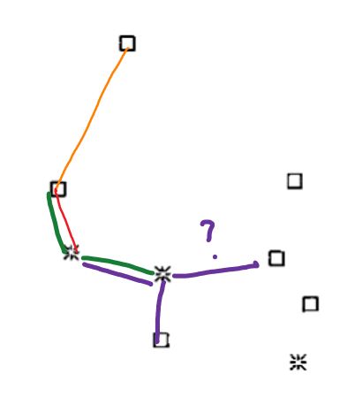
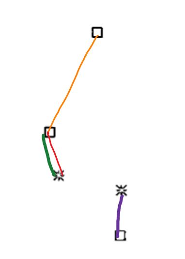
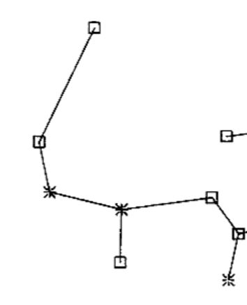
I was thinking that when creating the MST and creating the edges to the nodes, you should take the minimal value of euclidean distance. But for example, in figure 1b, there is nodes that are closer to a node, but however, their edge goes to other point, for example:
In this case, we can connect the points withing this options;
And then we will have this result:
But instead of that, the figure show us that the correct way to do it is to do it this way:
And I don't understand why. Maybe becuase you can't link twice nodes? That will make sense but I don't find where is that mentioned in the paper.