After implementing Sugar & James jump method and applying it straightforwardly to a few data sets, we're ready to throw it a few curveballs. This will demonstrate both its robustness and some necessary aspects of setting it up for success.
Again we need some functions we built in part one and part two. Feel free to skip this part if you don't need the review and you're not following along with a REPL. If you are following along in the REPL, here's the full Clojure source.
(def iris (i/to-matrix (incd/get-dataset :iris)))

(defn assoc-distortions
  "Given a number `transformation-power-y` and a seq of maps
  `clusterers`, where each map describes a k-means clusterer, return a
  seq of maps describing the same clusterers, now with key :distortion
  mapped to the value of the cluster analysis' squared error raised to
  the negative `transformation-power-y`.

  Based on Sugar & James' paper at
  http://www-bcf.usc.edu/~gareth/research/ratedist.pdf which defines
  distortion (denoted d[hat][sub k]) for a given k as the mean squared error when covariance
  is the identity matrix. This distortion is then transformed by
  raising it to the negative of the transformation power y, which is
  generally set to the number of attributes divided by two."
  [clusterers transformation-power-y]
  (map #(assoc % :distortion (Math/pow (:squared-error %) (- transformation-power-y)))
       clusterers))

(defn assoc-jumps
  "Given a seq of maps `clusterers` each describing a k-means analysis
  including the transformed :distortion of that analysis, returns a
  sequence of maps 'updated' with the calculated jumps in transformed
  distortions.

  Based on Sugar & James' paper at
  http://www-bcf.usc.edu/~gareth/research/ratedist.pdf which defines
  the jump for a given k (denoted J-sub-k) as simply the transformed distortion for k
  minus the transformed distortion for k-1."
  [clusterers]
  (map (fn [[a b]] (assoc b :jump (- (:distortion b) (:distortion a))))
       (partition 2 1 (conj clusterers {:distortion 0}))))

(def abc-keys
  "Returns a function that, given integer `n`, returns a seq of
  alphabetic keys. Only valid for n<=26."
  (let [ls (mapv (comp keyword str) "abcdefghikjlmnopqrstuvwxyz")]
    (fn [n] (take n ls))))

(def init-codes
  {:random 0
   :k-means++ 1
   :canopy 2
   :farthest-first 3})

(defn clusterer-over-k
  "Returns a k-means clusterer built over the `dataset` (which we call
  `ds-name`), using `k` number of clusters."
  [dataset ds-name k init-method]
  (mlc/clusterer-info
   (doto (mlc/make-clusterer :k-means
                             {:number-clusters k
                              :initialization-method (init-codes init-method)})
     (.buildClusterer (mld/make-dataset ds-name
                                        (abc-keys (count (first dataset)))
                                        dataset)))))

(defn clusterers-over-ks
  "Returns a seq of k-means clusterer objects that have been built on
  the given `dataset` that we call `ds-name`, where for each k in
  0<k<`max-k` one clusterer attempts to fit that number of clusters to
  the data. Optionally takes a map of `options` according to clj-ml's
  `make-clusterer`."
  [dataset ds-name max-k init-method]
  (map #(clusterer-over-k dataset ds-name % init-method)
       (range 1 (inc max-k))))

(defn graph-k-analysis
  "Performs cluster analyses using k=1 to max-k, graphs a selection of
  comparisons between those choices of k, and returns a JFree chart
  object. Requires the `dataset` as a vector of vectors, the name of
  the data set `ds-name`, the greatest k desired for analysis `max-k`,
  the transformation power to use `y`, the desired initial centroid
  placement method `init-method` as a keyword from the set
  #{:random :k-means++ :canopy :farthest-first}, and a vector of keys
  describing the `analyses` desired, which must be among the set
  #{:squared-errors, :distortions, :jumps}."
  [dataset ds-name max-k y init-method analyses]
  {:pre (seq (init-codes init-method))}
  (let [clusterers (clusterers-over-ks dataset ds-name max-k init-method)
        clusterer-distortions (assoc-distortions clusterers y)]
    (when (some #{:squared-errors} analyses)
      (i/view (incc/line-chart (map :number-clusters clusterers)
                               (map :squared-error clusterers)
                               :title (str ds-name ": SSE according to selection of k")
                               :x-label "Number of clusters, k"
                               :y-label "Within-cluster sum of squared errors")))
    (when (some #{:distortions} analyses)
      (i/view (incc/line-chart (map :number-clusters clusterer-distortions)
                               (map :distortion clusterer-distortions)
                               :title (str ds-name ": Distortions according to k")
                               :x-label "Number of clusters, k"
                               :y-label (str "Transformed distortions, J, using y=" y))))
    (when (some #{:jumps} analyses)
      (i/view (incc/line-chart (map :number-clusters (assoc-jumps clusterer-distortions))
                               (map :jump (assoc-jumps clusterer-distortions))
                               :title (str ds-name ": Jumps according to k")
                               :x-label "Number of clusters, k"
                               :y-label (str "Jumps in transformed distortions, J, using y=" y))))))

(defn gaussian-point
  [[x y] sd]
  [(incs/sample-normal 1 :mean x :sd sd)
(incs/sample-normal 1 :mean y :sd sd)])For our next trick we'll create a data set of 9 clusters. But these 9 clusters will themselves be clustered in groups of 3. This replica of Figure 3 in Sugar & James' paper
provides an example of a data set for which not only do the jump and broken line methods work well but using the raw distortion curve fails.
(def coordinates [[0   0] [1   0] [0.5 1]
                  [2.5 4] [3   5] [3.5 4]
                  [5   0] [5.5 1] [6   0]])

(def nine-gaussians
  (mapcat (fn [coords] (repeatedly 25 #(gaussian-point coords 0.1)))
          coordinates))
...and we take a look:
(i/view (incc/scatter-plot (map first nine-gaussians)
                           (map second nine-gaussians)
                           :title "A simulated data set with nine Gaussian clusters [Figure 3a]"))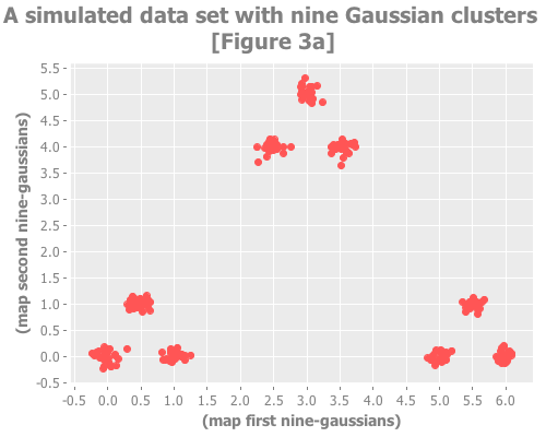
...and we look at the distortions and jumps:
(graph-k-analysis nine-gaussians "Nine Gaussians" 12 1 :random
                  [:squared-errors :jumps])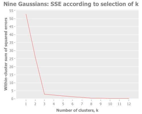
This is a great example of how the elbow method fails for data sets in which clusters are grouped hierarchically. One can see the 3 mega-clusters but not the 9 that make them up.
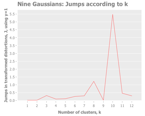
Screeeeech! Something—perhaps the jump method?—has gone off the rails. With 25 Cartesian points around each Gaussian point, using :random initial centroid placement, the jump method tells me that my WEKA k-means runs are definitely converging on k=10. Yet we know k is most certainly either 9 or 3. (Since the elbow method went all-in on the least value of k that shows a change, it seems to avoid this failure mode; the difference of opinion is between 9 and 10, not 3 and 9.)
Let's debug this little k=10 oddity. Could it be caused by our choice of transformation power, y?
(graph-k-analysis nine-gaussians "Nine Gaussians with y=1.5"
                  12 1.5 :random [:jumps])
(graph-k-analysis nine-gaussians "Nine Gaussians with y=0.5"
                  12 0.5 :random [:jumps])
(graph-k-analysis nine-gaussians "Nine Gaussians with y=0.33"
                  12 0.33 :random [:jumps])
(graph-k-analysis nine-gaussians "Nine Gaussians with y=0.25"
                  12 0.25 :random [:jumps])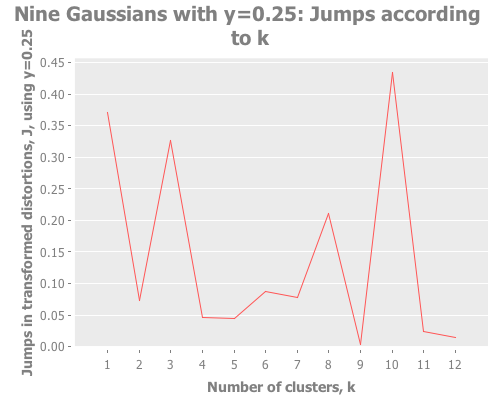
(graph-k-analysis nine-gaussians "Nine Gaussians with y=0.2"
                  12 0.2 :random [:jumps])
Y certainly doesn't seem to be the problem. What I see is that k=10 and other values dominate, whereas k=9 is actually the lowest result. So, k-means is simply converging strongly on k=10 and very much not converging on k=9. What else could cause this? It happens across multiple re-defs of nine-gaussians, so we can't blame it on a fluke of random distribution. Let's drop down out of "analysis mode" regarding distortions and jumps and just look at these weird clusters our algorithm is finding.
Here's a function that will run a k-means analysis and then graph the clusters it finds. As with previous (defn)s, I'm taking previously written exploratory code and repurposing it for reuse. Note that I'm not performing any PCA, so this only handles 2-dimensional data sets.
(defn see-clusters
  "Given a vector of vectors of 2-dimensional numerical `data` (i.e.,
  principal component analysis, if necessary, must be performed
  elsewhere), an integer number of clusters to visualize `k`, and an
  integer seed value for the random number generator, this function
  uses Incanter to graph a WEKA k-means clustering attempt on data
  using a random seed, with each cluster its own color."
  [data k]
  (let [k-means-clusterer (doto (mlc/make-clusterer :k-means
                                                    {:number-clusters k
                                                     :preserve-instances-order true})
                            (.buildClusterer
                             (mld/make-dataset "Cluster Visualization"
                                               (abc-keys (count (first data)))
                                               data)))
        data-clustered (map conj data (.getAssignments k-means-clusterer))]
    (i/save (incc/scatter-plot (map first data-clustered)
                               (map second data-clustered)
                               :legend true
                               :group-by (map last data-clustered)
                               :title "Visualizing clusters")
            "nine-wrongly-clustered-9.png")))

(see-clusters nine-gaussians 9) ;; set k to the known-correct number of clusters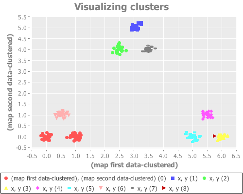
(see-clusters nine-gaussians 10) ;; set k to the answer WEKA's algorithm is arriving at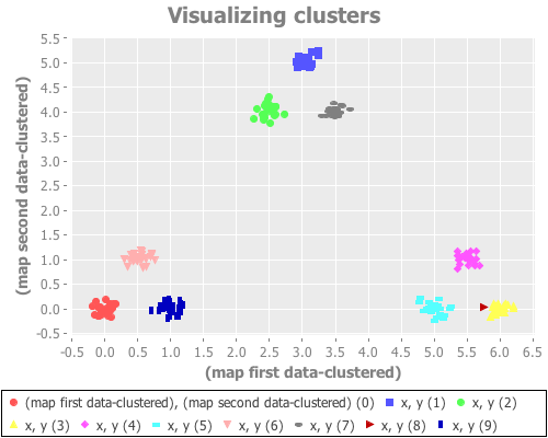
What I see for k=9 is every cluster appropriately grouped...except two Gaussian points are classified together as one cluster, and another single Gaussian point is split into two clusters. For k=10 I see every Gaussian point assigned its own cluster, except for one that is split into two. This happens repeatedly over many re-definitions of nine-gaussians. (If you're evaling this at home in your own REPL, you may not get precisely what I get, due to differences in random distributions. But it should be similar.)
K-means is simply not converging on the correct clusters. This saves Sugar & James' jump method from indictment, since it accurately reports what k-means did:
In some of the simulations the jump approach occasionally incorrectly chose a very large number of clusters. It appears that the method can be somewhat sensitive to a non-optimal fit of the k-means algorithm.
To my mind, that's good. I'm not looking for my analytic tool to give me a different answer from my clustering tool. I like that the jump method is telling me more clearly what k-means is doing compared to the elbow method, even when k-means is speaking gibberish.
Anyway, what's almost certainly causing these malconverged clusters is a poor initial placement of cluster centroid guesses, leading those centroids to converge on local but not global minima. (K-means is highly dependent on initial centroid placement.) WEKA allows us to randomize those initial placements by passing a seed value. Let's revise (see-clusters) to add it:
(defn see-clusters
  "Given a vector of vectors of 2-dimensional numerical `data` (i.e.,
  principal component analysis, if necessary, must be performed
  elsewhere), an integer number of clusters to visualize `k`, and an
  integer seed value for the random number generator, this function
  uses Incanter to graph a WEKA k-means clustering attempt on data
  using a random seed, with each cluster its own color."
  [data k seed] ;; <--- accept a seed parameter (must be an integer)
  (let [k-means-clusterer (doto (mlc/make-clusterer :k-means
                                                    {:number-clusters k
                                                     ;; Pass the seed to WEKA:
                                                     :random-seed seed
                                                     :preserve-instances-order true})
                            (.buildClusterer
                             (mld/make-dataset "Cluster Visualization"
                                               (abc-keys (count (first data)))
                                               data)))
        data-clustered (map conj data (.getAssignments k-means-clusterer))]
    (i/view (incc/scatter-plot (map first data-clustered)
                               (map second data-clustered)
                               :legend true
                               :group-by (map last data-clustered)
                               :title "Visualizing clusters"))))

(see-clusters nine-gaussians 9 1)
(see-clusters nine-gaussians 9 5)
(see-clusters nine-gaussians 9 8)
(see-clusters nine-gaussians 9 9)
(see-clusters nine-gaussians 9 10)
(see-clusters nine-gaussians 9 11)
(see-clusters nine-gaussians 9 15)
(see-clusters nine-gaussians 9 25)
(see-clusters nine-gaussians 9 100)
(see-clusters nine-gaussians 9 500)
(see-clusters nine-gaussians 9 1000)
I'm not going to bore you with a dozen nearly identical scatter plots, but my results aren't any better with any of these seeds. Occasionally one will converge on k=9, but it's rare—on the order of 1 in 10 or 20. I think we can reject the seed parameter as the cause of our trouble here.
I still suspect, however, that it's the initial placement of cluster centroids that is fouling up our k-means runs here. (Spoiler alert: it is.) I'd like to prove it by using an initial placement method other than random, which we've been using until now with init-codes and passing :random to our graph-k-analysis function. In fact, at the time of this writing, if you use the latest release of clj-ml, it doesn't matter what initialization method you pass, because it will get ignored and random initialization used anyway. Fixing this took a pull request to clj-ml to make available the other three initialization methods that WEKA offers. Having done so I can now direct WEKA to place those initial centroids using either the k-means++ approach, or the canopy method, or the farthest-first method. Let's add that parameter in one final take on (see-clusters):
(defn see-clusters
  "Given a vector of vectors of 2-dimensional numerical `data` (i.e.,
  principal component analysis, if necessary, must be performed
  elsewhere), an integer number of clusters to visualize `k`, and an
  integer seed value for the random number generator, this function
  uses Incanter to graph a WEKA k-means clustering attempt on data
  using a random seed, with each cluster its own color."
  [data k init-method]
  {:pre (seq (init-codes init-method))}
  (let [k-means-clusterer (doto (mlc/make-clusterer
                                 :k-means
                                 {:number-clusters k
                                  ;; Kept for when user selects random init:
                                  :random-seed (rand-int 1000)
                                  :initialization-method (init-codes init-method)
                                  :preserve-instances-order true})
                            (.buildClusterer
                             (mld/make-dataset "Cluster Visualization"
                                               (abc-keys (count (first data)))
                                               data)))
        data-clustered (map conj data (.getAssignments k-means-clusterer))]
    (i/view (incc/scatter-plot (map first data-clustered)
                               (map second data-clustered)
                               :legend true
                               :group-by (map last data-clustered)
                               :title "Visualizing clusters"))))
This next part is important: you have to use a version of clj-ml that supports initialization-method as an option for make-clusterer. If you don't, you'll get identical results across all four initialization methods we're about to use. (Sidebar: I am not a fan of silently failing when passed an invalid keyword option. 'Tis better to throw an error than for me to suffer the slings and arrows of outrageous goose chases because of a typo or misconfiguration.)
The simplest way I know of to do this at the moment uses the process described by Rafal Spacjer, which in this circumstance means:
- Clone my fork of clj-ml or, since my PR was accepted but a new version has not been released, the latest clj-ml from GitHub to your machine
- In that cloned clj-ml project, change the version in
project.cljto "0.6.1-SNAPSHOT" and save the file. This keeps things nice and clean so you can switch between the modified version and the official version. - Run
lein installfrom inside that cloned project directory. This creates a local repository that you can now add a dependency for in the project.clj of this project. - In this project's project.clj, swap this dependency:
[cc.artifice/clj-ml "0.6.1"]for this one:[cc.artifice/clj-ml "0.6.1-SNAPSHOT"]and save the file. - Finally, restart CIDER and re-evaluate your way back to this spot. You should now see different results from evaluating in the following four sexps.
(see-clusters nine-gaussians 9 :random)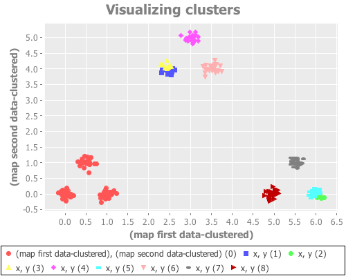
Random initial placements performs consistently poorly, as one would expect from prior experimentation.
(see-clusters nine-gaussians 9 :k-means++)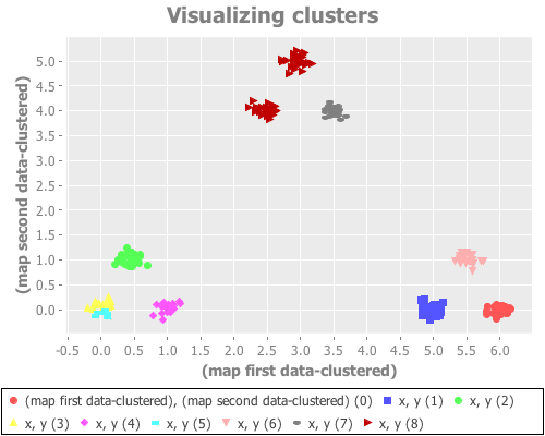
k-means++ initialization works by choosing the first centroid randomly from the points of the data set, then subsequently picking from the remaining points with probability corresponding to distance from the nearest cluster centroid. In my experimentation it seems with most instantiations of nine-gaussians to rarely converge correctly, but (not having tested this rigorously) to do so slightly more often than the random approach. (With some defs of nine-gaussians k-means++ leads us to correct clustering fairly often, but I found it rather fragile in this regard.)
(see-clusters nine-gaussians 9 :canopy)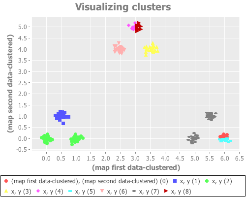
The canopy method is actually its own clustering algorithm, but is often used as a quick-and-dirty "pre-clustering" tool, as we do here. Without getting into the details of its algorithm, we use it as a computationally efficient way to approximately place centroids before switching to the more rigorous k-means process. For this data set, I saw results no better than k-means++. (Again, I did not test this rigorously. We're just exploring.)
(see-clusters nine-gaussians 9 :farthest-first)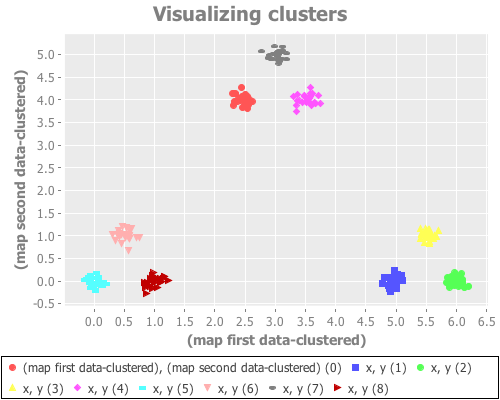
Yeeeeeeeehaw! Now we're cooking with apparently effective initial centroid placements for this particular data set!
The farthest-first method picks its first data point randomly, then chooses each successive point by finding the data point furthest from all the already-traversed data points. Once k points have been chosen, k-means is used to iteratively find clusters. (If one simply assigns the remaining points to the nearest centroid instead of switching to k-means, farthest-first can be used as its own clustering algorithm.) This hybrid approach seems to work very, very well on this data set. Interestingly, it seems to return the same result across dozens of runs, regardless of seeding.
Now that we've found an initial centroid placement method that doesn't fall flat on its face when asked to find 9 clusters on this data set, let's return to our original problem: evaluating selection of k. Let's just pass this successful initialization method to our graphing function:
(graph-k-analysis nine-gaussians "Nine Gaussians" 12 1 :farthest-first [:jumps])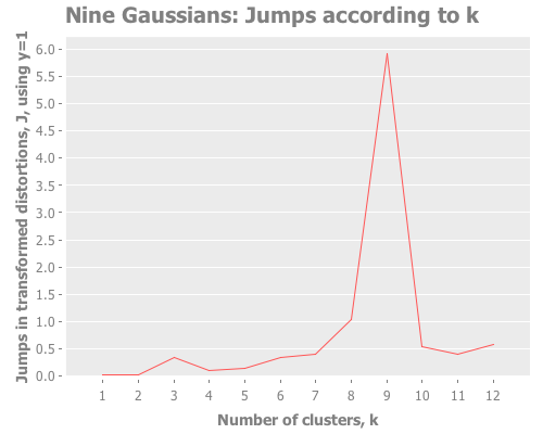
Now that's what I'm talking about. Once initialized properly, the jump method nails it for the "three clusters of three" curveball. It even picks up the secondary spike at k=3, though it does that better at slightly lower y values:
(graph-k-analysis nine-gaussians "Nine Gaussians" 12 (/ 1 2) :farthest-first [:jumps])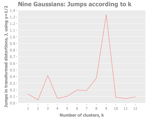
I wonder...how does initializing with farthest-first fare with the other data sets we've been looking at?
Iris data with Y=2/3:
(graph-k-analysis (i/to-vect (i/sel iris :cols (range 4))) "Fisher's Iris Data"
                  10 (/ 2 3) :farthest-first [:jumps])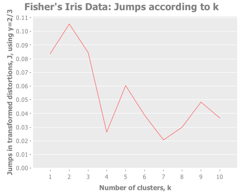
...with Y=1:
(graph-k-analysis (i/to-vect (i/sel iris :cols (range 4))) "Fisher's Iris Data"
                  10 1 :farthest-first [:jumps])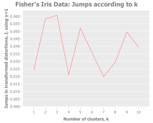
Taking these iris results collectively, the quality of farthest-first's performance is similar to that of random initial centroid placement. Interesting. The same seems to be true when we revisit the single gaussian point, which I provide again here so it's easy to re-define multiple times. Let's look at all four initialization methods:
(let [one-gaussian (apply map vector
                          (repeatedly 5 #(incs/sample-normal 300 :mean 1 :sd 1)))
      X-g (i/sel (i/to-matrix (i/to-dataset one-gaussian)) :cols (range 5))]
  (i/view (incc/scatter-plot (i/mmult X-g (i/sel (:rotation (incs/principal-components X-g))
                                                 :cols 0))
                             (i/mmult X-g (i/sel (:rotation (incs/principal-components X-g))
                                                 :cols 1))
                             :x-label "PC1" :y-label "PC2"
                             :title "Single-Gaussian PCA"))
  (graph-k-analysis one-gaussian "One Gaussian (init: random)" 10 (/ 5 2)
                    :random [:jumps])
  (graph-k-analysis one-gaussian "One Gaussian (init: k-means++)" 10 (/ 5 2)
                    :k-means++ [:jumps])
  (graph-k-analysis one-gaussian "One Gaussian (init: canopy)" 10 (/ 5 2)
                    :canopy [:jumps])
  (graph-k-analysis one-gaussian "One Gaussian (init: farthest-first)" 10 (/ 5 2)
                    :farthest-first [:jumps]))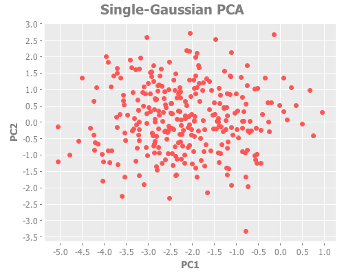
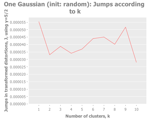
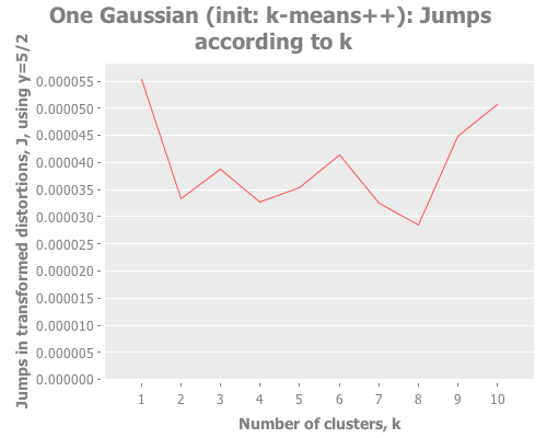
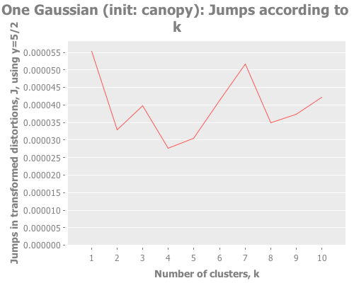
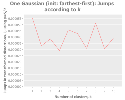
For brevity, I only present here one iteration, but those of you following along at home can eval and re-eval as you like, to get a better feel for the process. I see repeatedly for each initialization method across several runs is that two values of k do well: 1, and some value >5. Sometimes k=1 beats the greater value, sometimes not.
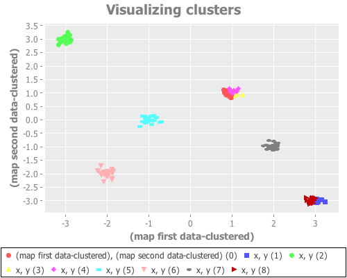
(let [six-gaussians (mapcat (fn [xc yc] (map (fn [x y] (vector x y))
                                            (incs/sample-normal 25 :mean xc :sd 0.1)
                                            (incs/sample-normal 25 :mean yc :sd 0.1)))
                            [-3 -2 -1 1  2  3]
                            [ 3 -2  0 1 -1 -3])]
  (i/view (incc/scatter-plot (map first six-gaussians)
                             (map second six-gaussians)
                             :title "Six Gaussians"))
  (graph-k-analysis six-gaussians "Six Gaussians (init: farthest-first)" 10 1
                    :farthest-first [:jumps])
  (graph-k-analysis six-gaussians "Six Gaussians (init: random)" 10 1
                    :random [:jumps])
  (graph-k-analysis six-gaussians "Six Gaussians (init: k-means++)" 10 1
                    :k-means++ [:jumps])
  (graph-k-analysis six-gaussians "Six Gaussians (init: canopy)" 10 1
                    :canopy [:jumps]))
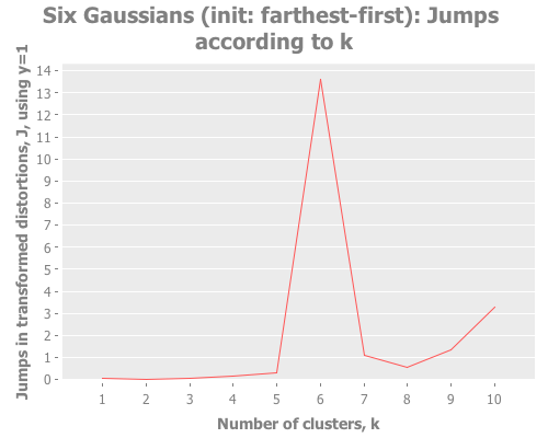
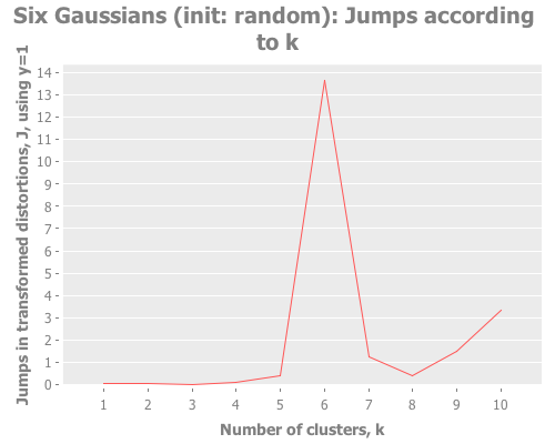
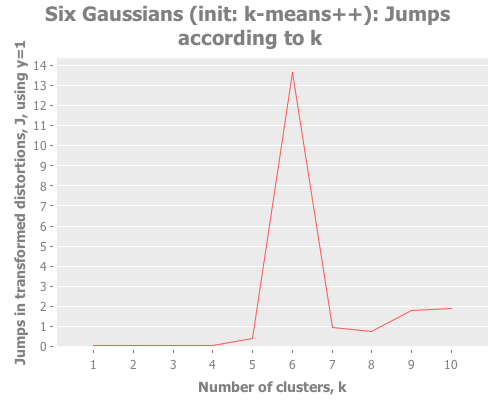
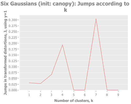
Fascinating. Canopy repeatedly crashes and burns, converging on something like k=7 or k=9, whereas all the other methods converge to k=6 easily. But look at the magnitude of those jump graphs: canopy's max jumps are on the order of 0.3, whereas the others are on the order of 13. Quelle difference! Watching this canopy collapse is mildly interesting:
(let [six-gaussians (mapcat (fn [xc yc] (map (fn [x y] (vector x y))
                                            (incs/sample-normal 25 :mean xc :sd 0.1)
                                            (incs/sample-normal 25 :mean yc :sd 0.1)))
                            [-3 -2 -1 1  2  3]
                            [ 3 -2  0 1 -1 -3])]
  (see-clusters six-gaussians 6 :canopy)
  (see-clusters six-gaussians 7 :canopy)
  (see-clusters six-gaussians 9 :canopy))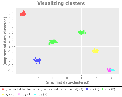

Anyway. I don't feel much need to chase down that rabbit hole: canopy does poorly with this sample data. Happens to the best of us.
OK. Whew! What have we learned trying to find clusters in the nine-points curveball of a data set? Initial centroid placement is important. Some methods for it rely on random seeding, which you in those cases need to take into account. Sometimes, some initialization methods crash and burn with a given data set, or only one will excel at a given data set. Yet, often, all four used here will perform similarly. When something goes wrong it can help to see its failure mode visually. Getting a feel for analysis of random distributions requires multiple runs. The jump method is often more insightful than the elbow method, especially when sub-grouping is present. Comparing magnitudes of jumps between separate runs is just like comparing magnitudes within the same run: it points you to the more convincing peaks in the jump graph.
Groovy. There's more to come in the fourth and final part, where we'll fight to defeat the forces of uncertainty and misleadingly aberrant results.