-
-
Save dfsnow/6cef8184ed0dbccadc0cd56a0d22b8be to your computer and use it in GitHub Desktop.
| ##### Setup ##### | |
| # Load the necessary libraries | |
| library(tidytransit) # Parse GTFS feeds | |
| library(dplyr) | |
| library(tidyr) | |
| library(lubridate) | |
| library(sf) | |
| library(ggplot2) | |
| library(gganimate) # Animate the ggplot + tween between frames | |
| library(ggspatial) # Add map tiles | |
| library(stinepack) # Interpolate between stop times | |
| # Set some simple parameters for the script | |
| feed <- "CTA GTFS" # Feed list can be found at tidytransit::feedlist | |
| transit_type = 1 # See tidytransit::route_type_names | |
| # Geographic area to plot. See boundingbox.klokantech.com for tool | |
| bbox <- c(-87.736558, 41.807137, -87.556657, 41.943711) | |
| # Trip departure date and times. Note that these are local time | |
| dep_date = lubridate::today() - days(1) | |
| min_dep_time = "08:00:00" | |
| max_arv_time = "09:00:00" | |
| # Animation length scalar. Smaller = shorter animation | |
| # A value of 1 means 1 minute of animation per hour depending on fps | |
| min_to_hour_ratio = 0.25 | |
| # Animation FPS. Higher values = smoother anim. but bigger file | |
| frames_per_second = 60 | |
| ##### Get GTFS feed ##### | |
| # Download a GTFS feed and parse it with tidytransit | |
| gtfs <- tidytransit::feedlist %>% | |
| filter(t == feed) %>% | |
| pull(url_d) %>% | |
| read_gtfs() | |
| # Keep only the routes (and corresponding trips and stops) specified | |
| route_ids <- gtfs$routes %>% | |
| filter(route_type == transit_type) %>% | |
| pull(route_id) | |
| trip_ids <- gtfs$trips %>% | |
| filter(route_id %in% route_ids) %>% | |
| pull(trip_id) | |
| stop_ids <- gtfs$stop_times %>% | |
| filter(trip_id %in% trip_ids) %>% | |
| pull(stop_id) %>% | |
| unique() | |
| # Load the static shapes of the routes and stops | |
| gtfs_sf <- gtfs %>% | |
| tidytransit::gtfs_as_sf() | |
| route_shapes <- gtfs_sf %>% | |
| get_route_geometry(route_ids) %>% | |
| left_join(gtfs$routes, by = "route_id") %>% | |
| mutate(route_color = paste0("#", route_color)) | |
| stop_shapes <- gtfs_sf$stops %>% | |
| filter(stop_id %in% stop_ids) | |
| ##### Get interpolated trips ##### | |
| # Each route is actually a series of points (held in the shapes | |
| # section of the feed) that are joined into a line. We can use | |
| # these points to define the waypoints that vehicles need to follow | |
| route_waypoints <- gtfs$trips %>% | |
| filter(route_id %in% route_ids) %>% | |
| distinct(route_id, shape_id) %>% | |
| left_join(gtfs$shapes, by = "shape_id") %>% | |
| select(-shape_pt_sequence) %>% | |
| rename( | |
| lat = shape_pt_lat, | |
| lon = shape_pt_lon, | |
| dist = shape_dist_traveled | |
| ) | |
| # Create a data frame of stops with time stopped and geographic | |
| # location. Only include trips within the time boundaries | |
| # specified at top of script | |
| stops_df <- gtfs$trips %>% | |
| filter(route_id %in% route_ids) %>% | |
| inner_join( | |
| filter_stop_times(gtfs, dep_date, min_dep_time, max_arv_time), | |
| by = "trip_id" | |
| ) %>% | |
| inner_join(gtfs$stops, by = "stop_id") %>% | |
| distinct( | |
| route_id, shape_id, trip_id, arrival_time, | |
| lat = stop_lat, lon = stop_lon, dist = shape_dist_traveled | |
| ) | |
| # For each trip, get ALL the waypoints along the route | |
| # (basically the points between each stop for each trip) | |
| waypoints_df <- stops_df %>% | |
| distinct(trip_id, shape_id) %>% | |
| inner_join(route_waypoints, by = "shape_id") | |
| # Combine the known stop times with the unknown waypoint times, | |
| # then fill in the missing waypoint data with time-series | |
| # imputation based on the distance column | |
| final_df <- stops_df %>% | |
| bind_rows(waypoints_df) %>% | |
| group_by(trip_id) %>% | |
| filter(sum(!is.na(arrival_time)) > 1) %>% | |
| mutate( | |
| time = as.POSIXct( | |
| as.character(arrival_time), format = "%H:%M:%S", | |
| tz = gtfs$agency$agency_timezone | |
| ) - days(1) | |
| ) %>% | |
| arrange(trip_id, dist) %>% | |
| group_by(trip_id, dist) %>% | |
| filter(row_number() == 1) %>% | |
| group_by(trip_id) %>% | |
| mutate( | |
| time = as.POSIXct( | |
| stinepack::na.stinterp( | |
| as.numeric(time), | |
| along = dist, | |
| na.rm = FALSE | |
| ), | |
| origin = "1970-01-01", | |
| tz = gtfs$agency$agency_timezone | |
| ) | |
| ) %>% | |
| ungroup() %>% | |
| filter(!is.na(time)) | |
| ##### Create animation ##### | |
| # If bounding box is not set, will use bbox of routes | |
| if (!exists("bbox")) bbox <- st_bbox(route_shapes) | |
| # Create a plot object to animate. Removing annotation_map_tile() will | |
| # signficantly speed up drawing each frame | |
| p <- ggplot(route_shapes) + | |
| annotation_map_tile(type = "cartolight", zoomin = 0, progress = "none") + | |
| geom_sf(data = route_shapes, aes(color = route_color), size = 1.5) + | |
| geom_sf( | |
| data = stop_shapes, stroke = 1.5, | |
| size = 4, shape = 21, | |
| color = "#000000", fill = "#ffffff" | |
| ) + | |
| coord_sf(xlim = c(bbox[1], bbox[3]), ylim = c(bbox[2], bbox[4])) + | |
| geom_point( | |
| data = final_df, | |
| aes(x = lon, y = lat, group = trip_id), | |
| size = 2.5, | |
| shape = 15 | |
| ) + | |
| scale_color_identity() + | |
| transition_components(time) + | |
| ease_aes("sine-in-out") + | |
| theme_void() + | |
| labs( | |
| title = gtfs$agency$agency_name, | |
| subtitle = "{frame_time}") + | |
| theme( | |
| legend.position = "none", | |
| plot.title = element_text(face = "bold", size = 24), | |
| plot.subtitle = element_text(size = 18) | |
| ) | |
| # Create the actual frames of animation | |
| frames <- as.numeric(hms(max_arv_time) - hms(min_dep_time)) * min_to_hour_ratio | |
| plot_mg <- animate( | |
| plot = p, nframes = frames, fps = frames_per_second, | |
| width = 800, height = 800, | |
| device = "png", | |
| renderer = file_renderer(dir = ".", overwrite = TRUE) | |
| ) |
Seems like an update to tidytransit changed the parsing for arrival times. read_gtfs converts them to hms now instead of strings. You should be able to fix it by just converting the times back to strings before parsing them. Starting at line 115:
  mutate(
    time = as.POSIXct(
      arrival_time, format = "%H:%M:%S",
      tz = gtfs$agency$agency_timezone,
      origin
    ) - days(1)
  ) %>%
becomes:
  mutate(
    time = as.POSIXct(
      as.character(arrival_time), format = "%H:%M:%S",
      tz = gtfs$agency$agency_timezone,
      origin
    ) - days(1)
  ) %>%
Let me know if that fixes it. I'll update the gist.
HI @dfsnow thanks for getting back to me! That adjustment seemed to fix the issue when using the default departure date. However I have another issue now where if I change the date in Line 22 from dep_date = lubridate::today() - days(1) to another date like dept_date = ymd("20220615") The subtitle still displays yesterday's date. I tried to mess around with Lines 125-137 based on your explanation above but to no avail. Any ideas?
L119 is subtracting a day for a reason I can't remember at the moment. Try changing that line.
@dfsnow looks like when I remove that line it changes the date from yesterday to today. My current workaround for this issue is changing L132 from "1970-01-01" the equivalent number of days backwards or forwards from today date to the desired date (minus 1 if L119 is kept) For instance if today is 07/18/2022 and I want the title to display "06/15/2022" I change the date to "1969-11-30". Not the prettiest solution but I thought I'd throw that out there.
Hello Dan, great work on this gist, it has been very useful.
I work at a local government transport agency in Auckland, New Zealand. We would like to adapt this code to produce some visualizations for the public. I can't see a license for this code, may we use it to create derivative code and credit you as Dan Snow (http://sno.ws/)?
@TLDuhamel Glad to see people are getting some use from it! Consider it MIT licensed. Would love to see your results if you want to drop them in this thread once you're done!
Also note, I've been playing with a better version of this code for a bit with more features: actual stopping at stops, proper speed up + slow down, fixes for overlapping tracks, etc. I'll try to find some time in the next few weeks to write up a post about it.
@dfsnow I can now share the published animation, which was launched on Facebook: https://www.facebook.com/akltransport/videos/295156760023471/
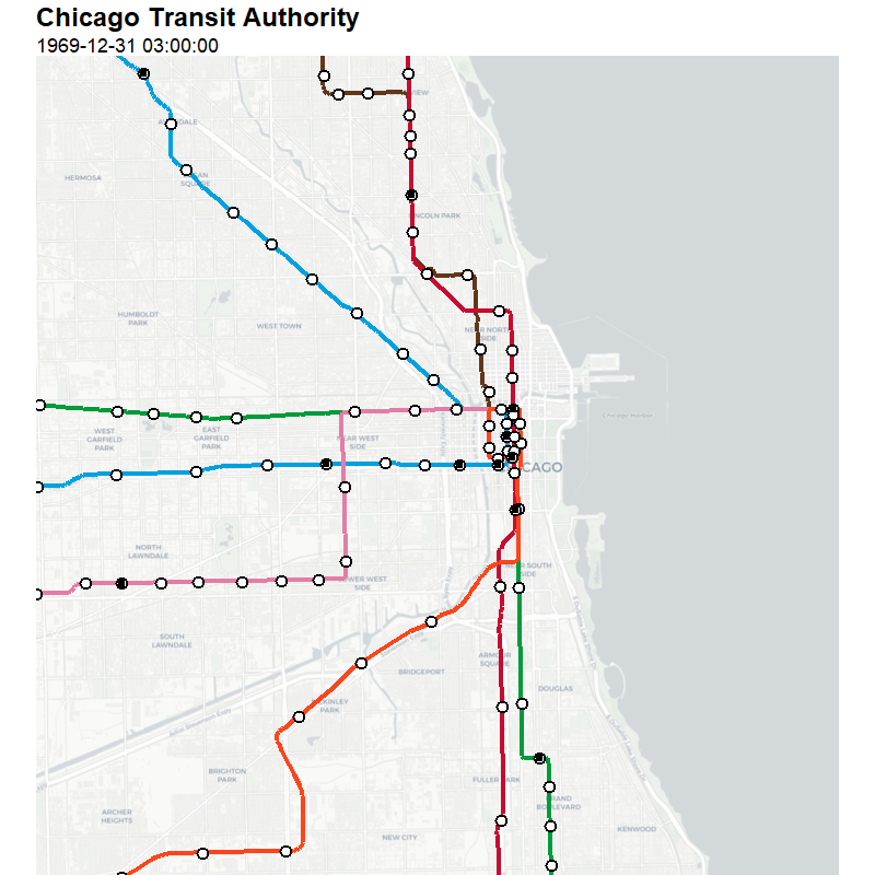
@dfsnow when running your example code here and using my own data, the default subtitle starts on December 31st, 1969 at 3:00:00. I believe it is animating the appropriate data for the correct "min_dep_time" to the "max_arv_time" but the date and time displayed in the subtitle is incorrect. I was able to get the date I want by changing the value in line 132 but still am lost on how to get the correct time to display. Am I missing something on how to get that to display correctly? My apologies if this question is not being asked correctly, I am new to GitHub. Any feedback would be very appreciated.